I previously took a lot of words to describe the guts of Markov chains and LLMs, and ended by pointing out that all LLMs can be split into two systems: one that takes in a list of tokens and outputs the probability of every possible token being the next one after, and a second that resolves those probabilities into a canonical next token. These two systems are independent, so in theory you could muck with any LLM by declaring an unlikely token to be the next one.
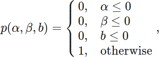
Few users are granted that fine level of control, but it’s common to be given two coarse dials to twiddle. The “temperature” controls the relative likelihood of tokens, while the “seed” changes the sequence of random values relied on by the second system. The former is almost always a non-negative real number, the latter an arbitrary integer.
Let’s take them for a spin.