If our goal is to raise funds for a good cause, we should at least have an idea of where the funds are at.
| created_at | amount | epoch | delta_epoch | culm | |
|---|---|---|---|---|---|
| 0 | 2017-01-24T07:27:51-06:00 | 10.0 | 2017-01-24 07:27:51-06:00 | -1218 days +19:51:12 | 14733.0 |
| 1 | 2017-01-24T07:31:09-06:00 | 50.0 | 2017-01-24 07:31:09-06:00 | -1218 days +19:54:30 | 14783.0 |
| 2 | 2017-01-24T07:41:20-06:00 | 100.0 | 2017-01-24 07:41:20-06:00 | -1218 days +20:04:41 | 14883.0 |
| 3 | 2017-01-24T07:50:20-06:00 | 10.0 | 2017-01-24 07:50:20-06:00 | -1218 days +20:13:41 | 14893.0 |
| 4 | 2017-01-24T08:03:26-06:00 | 25.0 | 2017-01-24 08:03:26-06:00 | -1218 days +20:26:47 | 14918.0 |
Changing the dataset so the last donation happens at time zero makes it both easier to fit the data and easier to understand what’s happening. The first day after the last donation is now day one.
Donations from 2017 don’t tell us much about the current state of the fund, though, so let’s focus on just the last year.
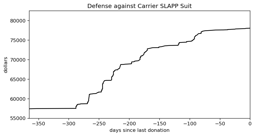
The donations seem to arrive in bursts, but there have been two quiet portions. One is thanks to the current pandemic, and the other was during last year’s late spring/early summer. It’s hard to tell what the donation rate is just by eye-ball, though. We need to smooth this out via a model.
The simplest such model is linear regression, aka. fitting a line. We want to incorporate uncertainty into the mix, which means a Bayesian fit. Now, what MCMC engine to use, hmmm…. emcee is my overall favourite, but I’m much too reliant on it. I’ve used PyMC3 a few times with success, but recently it’s been acting flaky. Time to pull out the big guns: Stan. I’ve been avoiding it because pystan‘s compilation times drove me nuts, but all the cool kids have switched to cmdstanpy when I looked away. Let’s give that a whirl.
CPU times: user 5.33 ms, sys: 7.33 ms, total: 12.7 ms
Wall time: 421 ms
CmdStan installed.
We can’t fit to the entire three-year time sequence, that just wouldn’t be fair given the recent slump in donations. How about the last six months? That covers both a few donation burts and a flat period, so it’s more in line with what we’d expect in future.
There were 117 donations over the last six months.
With the data prepped, we can shift to building the linear model.
I could have just gone with Stan’s basic model, but flat priors aren’t my style. My preferred prior for the slope is the inverse tangent, as it compensates for the tendency of large slope values to “bunch up” on one another. Stan doesn’t offer it by default, but the Cauchy distribution isn’t too far off.
We’d like the standard deviation to skew towards smaller values. It naturally tends to minimize itself when maximizing the likelihood, but an explicit skew will encourage this process along. Gelman and the Stan crew are drifting towards normal priors, but I still like a Cauchy prior for its weird properties.
Normally I’d plunk the Gaussian distribution in to handle divergence from the deterministic model, but I hear using Student’s T instead will cut down the influence of outliers. Thomas Wiecki recommends one degree of freedom, but Gelman and co. find that it leads to poor convergence in some cases. They recommend somewhere between three and seven degrees of freedom, but skew towards three, so I’ll go with the flow here.
The y-intercept could land pretty much anywhere, making its prior difficult to figure out. Yes, I’ve adjusted the time axis so that the last donation is at time zero, but the recent flat portion pretty much guarantees the y-intercept will be higher than the current amount of funds. The traditional approach is to use a flat prior for the intercept, and I can’t think of a good reason to ditch that.
Not convinced I picked good priors? That’s cool, there should be enough data here that the priors have minimal influence anyway. Moving on, let’s see how long compilation takes.
CPU times: user 4.91 ms, sys: 5.3 ms, total: 10.2 ms
Wall time: 20.2 s
This is one area where emcee really shines: as a pure python library, it has zero compilation time. Both PyMC3 and Stan need some time to fire up an external compiler, which adds overhead. Twenty seconds isn’t too bad, though, especially if it leads to quick sampling times.
CPU times: user 14.7 ms, sys: 24.7 ms, total: 39.4 ms
Wall time: 829 ms
And it does! emcee can be pretty zippy for a simple linear regression, but Stan is in another class altogether. PyMC3 floats somewhere between the two, in my experience.
Another great feature of Stan are the built-in diagnostics. These are really handy for confirming the posterior converged, and if not it can give you tips on what’s wrong with the model.
Processing csv files: /tmp/tmpyfx91ua9/linear_regression-202005262238-1-e393mc6t.csv, /tmp/tmpyfx91ua9/linear_regression-202005262238-2-8u_r8umk.csv, /tmp/tmpyfx91ua9/linear_regression-202005262238-3-m36dbylo.csv, /tmp/tmpyfx91ua9/linear_regression-202005262238-4-hxjnszfe.csv

Checking sampler transitions treedepth.
Treedepth satisfactory for all transitions.

Checking sampler transitions for divergences.
No divergent transitions found.

Checking E-BFMI - sampler transitions HMC potential energy.
E-BFMI satisfactory for all transitions.

Effective sample size satisfactory.

Split R-hat values satisfactory all parameters.

Processing complete, no problems detected.
The odds of a simple model with plenty of datapoints going sideways are pretty small, so this is another non-surprise. Enough waiting, though, let’s see the fit in action. First, we need to extract the posterior from the stored variables …
There are 256 samples in the posterior.
… and now free of its prison, we can plot the posterior against the original data. I’ll narrow the time window slightly, to make it easier to focus on the fit.
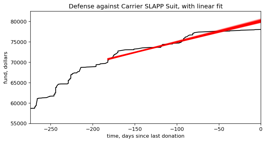
Looks like a decent fit to me, so we can start using it to answer a few questions. How much money is flowing into the fund each day, on average? How many years will it be until all those legal bills are paid off? Since humans aren’t good at counting in years, let’s also translate that number into a specific date.
mean/std/median slope = $51.62/1.65/51.76 per day

mean/std/median years to pay off the legal fees, relative to 2020-05-25 12:36:39-05:00 =
	1.962/0.063/1.955

mean/median estimate for paying off debt =
	2022-05-12 07:49:55.274942-05:00 / 2022-05-09 13:57:13.461426-05:00
Mid-May 2022, eh? That’s… not ideal. How much time can we shave off, if we increase the donation rate? Let’s play out a few scenarios.
median estimate for paying off debt, increasing rate by   1% = 2022-05-02 17:16:37.476652800
median estimate for paying off debt, increasing rate by   3% = 2022-04-18 23:48:28.185868800
median estimate for paying off debt, increasing rate by  10% = 2022-03-05 21:00:48.510403200
median estimate for paying off debt, increasing rate by  30% = 2021-11-26 00:10:56.277984
median estimate for paying off debt, increasing rate by 100% = 2021-05-17 18:16:56.230752
Bumping up the donation rate by one percent is pitiful. A three percent increase will almost shave off a month, which is just barely worthwhile, and a ten percent increase will roll the date forward by two. Those sound like good starting points, so let’s make them official: increase the current donation rate by three percent, and I’ll start pumping out the aforementioned blog posts on Bayesian statistics. Manage to increase it by 10%, and I’ll also record them as videos.
As implied, I don’t intend to keep the same rate throughout this entire process. If you surprise me with your generosity, I’ll bump up the rate. By the same token, though, if we go through a dry spell I’ll decrease the rate so the targets are easier to hit. My goal is to have at least a 50% success rate on that lower bar. Wouldn’t that make it impossible to hit the video target? Remember, though, it’ll take some time to determine the success rate. That lag should make it possible to blow past the target, and by the time this becomes an issue I’ll have thought of a better fix.
Ah, but over what timeframe should this rate increase? We could easily blow past the three percent target if someone donates a hundred bucks tomorrow, after all, and it’s no fair to announce this and hope your wallets are ready to go in an instant. How about… sixteen days. You’ve got sixteen days to hit one of those rate targets. That’s a nice round number, for a computer scientist, and it should (hopefully!) give me just enough time to whip up the first post. What does that goal translate to, in absolute numbers?
a 3% increase over 16 days translates to $851.69 + $78039.00 = $78890.69
Right, if you want those blog posts to start flowing you’ve got to get that fundraiser total to $78,890.69 before June 12th. As for the video…
a 10% increase over 16 days translates to $909.57 + $78039.00 = $78948.57
… you’ve got to hit $78,948.57 by the same date.
Ready? Set? Get donating!