Hello! I’ve been a fan of your work for some time. While I’ve used emcee more and currently use a lot of PyMC3, I love the layout of Stan‘s language and often find myself missing it.
But there’s no contradiction between being a fan and critiquing your work. And one of your recent blog posts left me scratching my head.
Suppose I want to estimate my chances of winning the lottery by buying a ticket every day. That is, I want to do a pure Monte Carlo estimate of my probability of winning. How long will it take before I have an estimate that’s within 10% of the true value?
This one’s pretty easy to set up, thanks to conjugate priors. The Beta distribution models our credibility of the odds of success from a Bernoulli process. If our prior belief is represented by the parameter pair \((\alpha_\text{prior},\beta_\text{prior})\), and we win \(w\) times over \(n\) trials, our posterior belief in the odds of us winning the lottery, \(p\), is
$$ \begin{align}
\alpha_\text{posterior} &= \alpha_\text{prior} + w, \\
\beta_\text{posterior} &= \beta_\text{prior} + n – w
\end{align} $$
You make it pretty clear that by “lottery” you mean the traditional kind, with a big payout that your highly unlikely to win, so \(w \approx 0\). But in the process you make things much more confusing.
There’s a big NY state lottery for which there is a 1 in 300M chance of winning the jackpot. Back of the envelope, to get an estimate within 10% of the true value of 1/300M will take many millions of years.
“Many millions of years,” when we’re “buying a ticket every day?” That can’t be right. The mean of the Beta distribution is
$$ \begin{equation}
\mathbb{E}[Beta(\alpha_\text{posterior},\beta_\text{posterior})] = \frac{\alpha_\text{posterior}}{\alpha_\text{posterior} + \beta_\text{posterior}}
\end{equation} $$
So if we’re trying to get that within 10% of zero, and \(w = 0\), we can write
$$ \begin{align}
\frac{\alpha_\text{prior}}{\alpha_\text{prior} + \beta_\text{prior} + n} &< \frac{1}{10} \\
10 \alpha_\text{prior} &< \alpha_\text{prior} + \beta_\text{prior} + n \\
9 \alpha_\text{prior} – \beta_\text{prior} &< n
\end{align} $$
If we plug in a sensible-if-improper subjective prior like \(\alpha_\text{prior} = 0, \beta_\text{prior} = 1\), then we don’t even need to purchase a single ticket. If we insist on an “objective” prior like Jeffrey’s, then we need to purchase five tickets. If for whatever reason we foolishly insist on the Bayes/Laplace prior, we need nine tickets. Even at our most pessimistic, we need less than a fortnight (or, if you prefer, much less than a Fortnite season). If we switch to the maximal likelihood instead of the mean, the situation gets worse.
$$ \begin{align}
\text{Mode}[Beta(\alpha_\text{posterior},\beta_\text{posterior})] &= \frac{\alpha_\text{posterior} – 1}{\alpha_\text{posterior} + \beta_\text{posterior} – 2} \\
\frac{\alpha_\text{prior} – 1}{\alpha_\text{prior} + \beta_\text{prior} + n – 2} &< \frac{1}{10} \\
9\alpha_\text{prior} – \beta_\text{prior} – 8 &< n
\end{align} $$
Now Jeffrey’s prior doesn’t require us to purchase a ticket, and even that awful Bayes/Laplace prior needs just one purchase. I can’t see how you get millions of years out of that scenario.
In the Interval
Maybe you meant a different scenario, though. We often use credible intervals to make decisions, so maybe you meant that the entire interval has to pass below the 0.1 mark? This introduces another variable, the width of the credible interval. Most people use two standard deviations or thereabouts, but I and a few others prefer a single standard deviation. Let’s just go with the higher bar, and start hacking away at the variance of the Beta distribution.
$$ \begin{align}
\text{var}[Beta(\alpha_\text{posterior},\beta_\text{posterior})] &= \frac{\alpha_\text{posterior}\beta_\text{posterior}}{(\alpha_\text{posterior} + \beta_\text{posterior})^2(\alpha_\text{posterior} + \beta_\text{posterior} + 2)} \\
\sigma[Beta(\alpha_\text{posterior},\beta_\text{posterior})] &= \sqrt{\frac{\alpha_\text{prior}(\beta_\text{prior} + n)}{(\alpha_\text{prior} + \beta_\text{prior} + n)^2(\alpha_\text{prior} + \beta_\text{prior} + n + 2)}} \\
\frac{\alpha_\text{prior}}{\alpha_\text{prior} + \beta_\text{prior} + n} + \frac{2}{\alpha_\text{prior} + \beta_\text{prior} + n} \sqrt{\frac{\alpha_\text{prior}(\beta_\text{prior} + n)}{\alpha_\text{prior} + \beta_\text{prior} + n + 2}} &< \frac{1}{10}
\end{align} $$
Our improper subjective prior still requires zero ticket purchases, as \(\alpha_\text{prior} = 0\) wipes out the entire mess. For Jeffrey’s prior, we find
$$ \begin{equation}
\frac{\frac{1}{2}}{n + 1} + \frac{2}{n + 1} \sqrt{\frac{1}{2}\frac{n + \frac 1 2}{n + 3}} < \frac{1}{10},
\end{equation} $$
which needs 18 ticket purchases according to Wolfram Alpha. The awful Bayes/Laplace prior can almost get away with 27 tickets, but not quite. Both of those stretch the meaning of “back of the envelope,” but you can get the answer via a calculator and some trial-and-error.
I used the term “hacking” for a reason, though. That variance formula is only accurate when \(p \approx \frac 1 2\) or \(n\) is large, and neither is true in this scenario. We’re likely underestimating the number of tickets we’d need to buy. To get an accurate answer, we need to integrate the Beta distribution.
$$ \begin{align}
\int_{p=0}^{\frac{1}{10}} \frac{\Gamma(\alpha_\text{posterior} + \beta_\text{posterior})}{\Gamma(\alpha_\text{posterior})\Gamma(\beta_\text{posterior})} p^{\alpha_\text{posterior} – 1} (1-p)^{\beta_\text{posterior} – 1} > \frac{39}{40} \\
40 \frac{\Gamma(\alpha_\text{prior} + \beta_\text{prior} + n)}{\Gamma(\alpha_\text{prior})\Gamma(\beta_\text{prior} + n)} \int_{p=0}^{\frac{1}{10}} p^{\alpha_\text{prior} – 1} (1-p)^{\beta_\text{prior} + n – 1} > 39
\end{align} $$
Awful, but at least for our subjective prior it’s trivial to evaluate. \(\text{Beta}(0,n+1)\) is a Dirac delta at \(p = 0\), so 100% of the integral is below 0.1 and we still don’t need to purchase a single ticket. Fortunately for both the Jeffrey’s and Bayes/Laplace prior, my “envelope” is a Jupyter notebook.
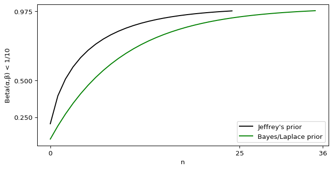
Those numbers did go up by a non-trivial amount, but we’re still nowhere near “many millions of years,” even if Fortnite’s last season felt that long.
Maybe you meant some scenario where the credible interval overlaps \(p = 0\)? With proper priors, that never happens; the lower part of the credible interval always leaves room for some extremely small values of \(p\), and thus never actually equals 0. My sensible improper prior has both ends of the interval equal to zero and thus as long as \(w = 0\) it will always overlap \(p = 0\).
Expecting Something?
I think I can find a scenario where you’re right, but I also bet you’re sick of me calling \((0,1)\) a “sensible” subjective prior. Hope you don’t mind if I take a quick detour to the last question in that blog post, which should explain how a Dirac delta can be sensible.
How long would it take to convince yourself that playing the lottery has an expected negative return if tickets cost $1, there’s a 1/300M chance of winning, and the payout is $100M?
Let’s say the payout if you win is \(W\) dollars, and the cost of a ticket is \(T\). Then your expected earnings at any moment is an integral of a multiple of the entire Beta posterior.
$$ \begin{equation}
\mathbb{E}(\text{Lottery}_{W}) = \int_{p=0}^1 \frac{\Gamma(\alpha_\text{posterior} + \beta_\text{posterior})}{\Gamma(\alpha_\text{posterior})\Gamma(\beta_\text{posterior})} p^{\alpha_\text{posterior} – 1} (1-p)^{\beta_\text{posterior} – 1} p W < T
\end{equation} $$
I’m pretty confident you can see why that’s a back-of-the-envelope calculation, but this is a public letter and I’m also sure some of those readers just fainted. Let me detour from the detour to assure them that, yes, this is actually a pretty simple calculation. They’ve already seen that multiplicative constants can be yanked out of the integral, but I’m not sure they realized that if
$$ \begin{equation}
\int_{p=0}^1 \frac{\Gamma(\alpha + \beta)}{\Gamma(\alpha)\Gamma(\beta)} p^{\alpha – 1} (1-p)^{\beta – 1} = 1,
\end{equation} $$
then thanks to the multiplicative constant rule it must be true that
$$ \begin{equation}
\int_{p=0}^1 p^{\alpha – 1} (1-p)^{\beta – 1} = \frac{\Gamma(\alpha)\Gamma(\beta)}{\Gamma(\alpha + \beta)}
\end{equation} $$
They may also be unaware that the Gamma function is an analytic continuity of the factorial. I say “an” because there’s an infinite number of functions that also qualify. To be considered a “good” analytic continuity the Gamma function must also duplicate another property of the factorial, that \((a + 1)! = (a + 1)(a!)\) for all valid \(a\). Or, put another way, it must be true that
$$ \begin{equation}
\frac{\Gamma(a + 1)}{\Gamma(a)} = a + 1, a > 0
\end{equation} $$
Fortunately for me, the Gamma function is a good analytic continuity, perhaps even the best. This allows me to chop that integral down to size.
$$ \begin{align}
W \frac{\Gamma(\alpha_\text{prior} + \beta_\text{prior} + n)}{\Gamma(\alpha_\text{prior})\Gamma(\beta_\text{prior} + n)} \int_{p=0}^1 p^{\alpha_\text{prior} – 1} (1-p)^{\beta_\text{prior} + n – 1} p &< T \\
\int_{p=0}^1 p^{\alpha_\text{prior} – 1} (1-p)^{\beta_\text{prior} + n – 1} p &= \int_{p=0}^1 p^{\alpha_\text{prior}} (1-p)^{\beta_\text{prior} + n – 1} \\
\int_{p=0}^1 p^{\alpha_\text{prior}} (1-p)^{\beta_\text{prior} + n – 1} &= \frac{\Gamma(\alpha_\text{prior} + 1)\Gamma(\beta_\text{prior} + n)}{\Gamma(\alpha_\text{prior} + \beta_\text{prior} + n + 1)} \\
W \frac{\Gamma(\alpha_\text{prior} + \beta_\text{prior} + n)}{\Gamma(\alpha_\text{prior})\Gamma(\beta_\text{prior} + n)} \frac{\Gamma(\alpha_\text{prior} + 1)\Gamma(\beta_\text{prior} + n)}{\Gamma(\alpha_\text{prior} + \beta_\text{prior} + n + 1)} &< T \\
W \frac{\Gamma(\alpha_\text{prior} + \beta_\text{prior} + n) \Gamma(\alpha_\text{prior} + 1)}{\Gamma(\alpha_\text{prior} + \beta_\text{prior} + n + 1) \Gamma(\alpha_\text{prior})} &< T \\
W \frac{\alpha_\text{prior} + 1}{\alpha_\text{prior} + \beta_\text{prior} + n + 1} &< T \\
\frac{W}{T}(\alpha_\text{prior} + 1) – \alpha_\text{prior} – \beta_\text{prior} – 1 &< n
\end{align} $$
Mmmm, that was satisfying. Anyway, for Jeffrey’s prior you need to purchase \(n > 149,999,998\) tickets to be convinced this lottery isn’t worth investing in, while the Bayes/Laplace prior argues for \(n > 199,999,997\) purchases. Plug my subjective prior in, and you’d need to purchase \(n > 99,999,998\) tickets.
That’s optimal, assuming we know little about the odds of winning this lottery. The number of tickets we need to purchase is controlled by our prior. Since \(W \gg T\), our best bet to minimize the number of tickets we need to purchase is to minimize \(\alpha_\text{prior}\). Unfortunately, the lowest we can go is \(\alpha_\text{prior} = 0\). Almost all the “objective” priors I know of have it larger, and thus ask that you sink more money into the lottery than the prize is worth. That doesn’t sit well with our intuition. The sole exception is the Haldane prior of (0,0), which argues for \(n > 99,999,999\) and thus asks you to spend exactly as much as the prize-winnings. By stating \(\beta_\text{prior} = 1\), my prior manages to shave off one ticket purchase.
Another prior that increases \(\beta_\text{prior}\) further will shave off further purchases, but so far we’ve only considered the case where \(w = 0\). What if we sink money into this lottery, and happen to win before hitting our limit? The subjective prior of \((0,1)\) after \(n\) losses becomes equivalent to the Bayes/Laplace prior of \((1,1)\) after \(n-1\) losses. Our assumption that \(p \approx 0\) has been proven wrong, so the next best choice is to make no assumptions about \(p\). At the same time, we’ve seen \(n\) losses and we’d be foolish to discard that information entirely. A subjective prior with \(\beta_\text{prior} > 1\) wouldn’t transform in this manner, while one with \(\beta_\text{prior} < 1\) would be biased towards winning the lottery relative to the Bayes/Laplace prior.
My subjective prior argues you shouldn’t play the lottery, which matches the reality that almost all lotteries pay out less than they take in, but if you insist on participating it will minimize your losses while still responding well to an unexpected win. It lives up to the hype.
However, there is one way to beat it. You mentioned in your post that the odds of winning this lottery are one in 300 million. We’re not supposed to incorporate that into our math, it’s just a measuring stick to use against the values we churn out, but what if we constructed a prior around it anyway? This prior should have a mean of one in 300 million, and the \(p = 0\) case should have zero likelihood. The best match is \((1+\epsilon, 299999999\cdot(1+\epsilon))\), where \(\epsilon\) is a small number, and when we take a limit …
$$ \begin{equation}
\lim_{\epsilon \to 0^{+}} \frac{100,000,000}{1}(2 + \epsilon) – 299,999,999 \epsilon – 300,000,000 = -100,000,000 < n
\end{equation} $$
… we find the only winning move is not to play. There’s no Dirac deltas here, either, so unlike my subjective prior it’s credible interval is one-dimensional. Eliminating the \(p = 0\) case runs contrary to our intuition, however. A newborn that purchased a ticket every day of its life until it died on its 80th birthday has a 99.99% chance of never holding a winning ticket. \(p = 0\) is always an option when you live a finite amount of time.
The problem with this new prior is that it’s incredibly strong. If we didn’t have the true odds of winning in our back pocket, we could quite fairly be accused of putting our thumb on the scales. We can water down \((1,299999999)\) by dividing both \(\alpha_\text{prior}\) and \(\beta_\text{prior}\) by a constant value. This maintains the mean of the Beta distribution, and while the \(p = 0\) case now has non-zero credence I’ve shown that’s no big deal. Pick the appropriate constant value and we get something like \((\epsilon,1)\), where \(\epsilon\) is a small positive value. Quite literally, that’s within epsilon of the subjective prior I’ve been hyping!
Enter Frequentism
So far, the only back-of-the-envelope calculations I’ve done that argued for millions of ticket purchases involved the expected value, but that was only because we used weak priors that are a poor match for reality. I believe in the principle of charity, though, and I can see a scenario where a back-of-the-envelope calculation does demand millions of purchases.
But to do so, I’ve got to hop the fence and become a frequentist.
If you haven’t read The Theory That Would Not Die, you’re missing out. Sharon Bertsch McGrayne mentions one anecdote about the RAND Corporation’s attempts to calculate the odds of a nuclear weapon accidentally detonating back in the 1950’s. No frequentist statistician would touch it with a twenty-foot pole, but not because they were worried about getting the math wrong. The problem was the math. As the eventually-published report states:
The usual way of estimating the probability of an accident in a given situation is to rely on observations of past accidents. This approach is used in the Air Force, for example, by the Directory of Flight Safety Research to estimate the probability per flying hour of an aircraft accident. In cases of of newly introduced aircraft types for which there are no accident statistics, past experience of similar types is used by analogy.
Such an approach is not possible in a field where this is no record of past accidents. After more than a decade of handling nuclear weapons, no unauthorized detonation has occurred. Furthermore, one cannot find a satisfactory analogy to the complicated chain of events that would have to precede an unauthorized nuclear detonation. (…) Hence we are left with the banal observation that zero accidents have occurred. On this basis the maximal likelihood estimate of the probability of an accident in any future exposure turns out to be zero.
For the lottery scenario, a frequentist wouldn’t reach for the Beta distribution but instead the Binomial. Given \(n\) trials of a Bernoulli process with probability \(p\) of success, the expected number of successes observed is
$$ \begin{equation}
\bar w = n p
\end{equation} $$
We can convert that to a maximal likelihood estimate by dividing the actual number of observed successes by \(n\).
$$ \begin{equation}
\hat p = \frac{w}{n}
\end{equation} $$
In many ways this estimate can be considered optimal, as it is both unbiased and has the least variance of all other estimators. Thanks to the Central Limit Theorem, the Binomial distribution will approximate a Gaussian distribution to arbitrary degree as we increase \(n\), which allows us to apply the analysis from the latter to the former. So we can use our maximal likelihood estimate \(\hat p\) to calculate the standard error of that estimate.
$$ \begin{equation}
\text{SEM}[\hat p] = \sqrt{ \frac{\hat p(1- \hat p)}{n} }
\end{equation} $$
Ah, but what if \(w = 0\)? It follows that \(\hat p = 0\), but this also means that \(\text{SEM}[\hat p] = 0\). There’s no variance in our estimate? That can’t be right. If we approach this from another angle, plugging \(w = 0\) into the Binomial distribution, it reduces to
$$ \begin{equation}
\text{Binomial}(w | n,p) = \frac{n!}{w!(n-w)!} p^w (1-p)^{n-w} = (1-p)^n
\end{equation} $$
The maximal likelihood of this Binomial is indeed \(p = 0\), but it doesn’t resemble a Dirac delta at all.
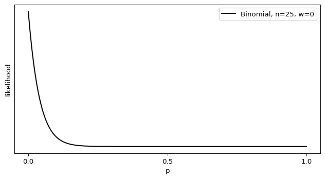
Shouldn’t there be some sort of variance there? What’s going wrong?
We got a taste of this on the Bayesian side of the fence. Using the stock formula for the variance of the Beta distribution underestimated the true value, because the stock formula assumed \(p \approx \frac 1 2\) or a large \(n\). When we assume we have a near-infinite amount of data, we can take all sorts of computational shortcuts that make our life easier. One look at the Binomial’s mean, however, tells us that we can drown out the effects of a large \(n\) with a small value of \(p\). And, just as with the odds of a nuclear bomb accident, we already know \(p\) is very, very small. That isn’t fatal on its own, as you correctly point out.
With the lottery, if you run a few hundred draws, your estimate is almost certainly going to be exactly zero. Did we break the [*Central Limit Theorem*]? Nope. Zero has the right absolute error properties. It’s within 1/300M of the true answer after all!
The problem comes when we apply the Central Limit Theorem and use a Gaussian approximation to generate a confidence or credible interval for that maximal likelihood estimate. As both the math and graph show, though, the probability distribution isn’t well-described by a Gaussian distribution. This isn’t much of a problem on the Bayesian side of the fence, as I can juggle multiple priors and switch to integration for small values of \(n\). Frequentism, however, is dependent on the Central Limit Theorem and thus assumes \(n\) is sufficiently large. This is baked right into the definitions: a p-value is the fraction of times you calculate a test metric equal to or more extreme than the current one assuming the null hypothesis is true and an infinite number of equivalent trials of the same random process, while confidence intervals are a range of parameter values such that when we repeat the maximal likelihood estimate on an infinite number of equivalent trials the estimates will fall in that range more often than a fraction of our choosing. Frequentist statisticians are stuck with the math telling them that \(p = 0\) with absolute certainty, which conflicts with our intuitive understanding.
For a frequentist, there appears to be only one way out of this trap: witness a nuclear bomb accident. Once \(w > 0\), the math starts returning values that better match intuition. Likewise with the lottery scenario, the only way for a frequentist to get an estimate of \(p\) that comes close to their intuition is to purchase tickets until they win at least once.
This scenario does indeed take “many millions of years.” It’s strange to find you taking a frequentist world-view, though, when you’re clearly a Bayesian. By straddling the fence you wind up in a world of hurt. For instance, you state this:
Did we break the [*Central Limit Theorem*]? Nope. Zero has the right absolute error properties. It’s within 1/300M of the true answer after all! But it has terrible relative error probabilities; it’s relative error after a lifetime of playing the lottery is basically infinity.
A true frequentist would have been fine asserting the probability of a nuclear bomb accident is zero. Why? Because \(\text{SEM}[\hat p = 0]\) is actually a very good confidence interval. If we’re going for two sigmas, then our confidence interval should contain the maximal likelihood we’ve calculated at least 95% of the time. Let’s say our sample sizes are \(n = 36\), the worst-case result from Bayesian statistics. If the true odds of winning the lottery are 1 in 300 million, then the odds of calculating a maximal likelihood of \(p = 0\) is
p( MLE(hat p) = 0 ) = 0.999999880000007
About 99.99999% of the time, then, the confidence interval of \(0 \leq \hat p \leq 0\) will be correct. That’s substantially better than 95%! Nothing’s broken here, frequentism is working exactly as intended.
I bet you think I’ve screwed up the definition of confidence intervals. I’m afraid not, I’ve double-checked my interpretation by heading back to the source, Jerzy Neyman. He, more than any other person, is responsible for pioneering the frequentist confidence interval.
We can then tell the practical statistician that whenever he is certain that the form of the probability law of the X’s is given by the function? \(p(E|\theta_1, \theta_2, \dots \theta_l,)\) which served to determine \(\underline{\theta}(E)\) and \(\bar \theta(E)\) [the lower and upper bounds of the confidence interval], he may estimate \(\theta_1\) by making the following three steps: (a) he must perform the random experiment and observe the particular values \(x_1, x_2, \dots x_n\) of the X’s; (b) he must use these values to calculate the corresponding values of \(\underline{\theta}(E)\) and \(\bar \theta(E)\); and (c) he must state that \(\underline{\theta}(E) < \theta_1^o < \bar \theta(E)\), where \(\theta_1^o\) denotes the true value of \(\theta_1\). How can this recommendation be justified?
[Neyman keeps alternating between \(\underline{\theta}(E) \leq \theta_1^o \leq \bar \theta(E)\) and \(\underline{\theta}(E) < \theta_1^o < \bar \theta(E)\) throughout this paper, so presumably both forms are A-OK.]
The justification lies in the character of probabilities as used here, and in the law of great numbers. According to this empirical law, which has been confirmed by numerous experiments, whenever we frequently and independently repeat a random experiment with a constant probability, \(\alpha\), of a certain result, A, then the relative frequency of the occurrence of this result approaches \(\alpha\). Now the three steps (a), (b), and (c) recommended to the practical statistician represent a random experiment which may result in a correct statement concerning the value of \(\theta_1\). This result may be denoted by A, and if the calculations leading to the functions \(\underline{\theta}(E)\) and \(\bar \theta(E)\) are correct, the probability of A will be constantly equal to \(\alpha\). In fact, the statement (c) concerning the value of \(\theta_1\) is only correct when \(\underline{\theta}(E)\) falls below \(\theta_1^o\) and \(\bar \theta(E)\), above \(\theta_1^o\), and the probability of this is equal to \(\alpha\) whenever \(\theta_1^o\) the true value of \(\theta_1\). It follows that if the practical statistician applies permanently the rules (a), (b) and (c) for purposes of estimating the value of the parameter \(\theta_1\) in the long run he will be correct in about 99 per cent of all cases. […]
It will be noticed that in the above description the probability statements refer to the problems of estimation with which the statistician will be concerned in the future. In fact, I have repeatedly stated that the frequency of correct results tend to \(\alpha\). [Footnote: This, of course, is subject to restriction that the X’s considered will follow the probability law assumed.] Consider now the case when a sample, E’, is already drawn and the calculations have given, say, \(\underline{\theta}(E’)\) = 1 and \(\bar \theta(E’)\) = 2. Can we say that in this particular case the probability of the true value of \(\theta_1\) falling between 1 and 2 is equal to \(\alpha\)?
The answer is obviously in the negative. The parameter \(\theta_1\) is an unknown constant and no probability statement concerning its value may be made, that is except for the hypothetical and trivial ones … which we have decided not to consider.
Neyman, Jerzy. “X — outline of a theory of statistical estimation based on the classical theory of probability.” Philosophical Transactions of the Royal Society of London. Series A, Mathematical and Physical Sciences 236.767 (1937): 348-349.
If there was any further doubt, it’s erased when Neyman goes on to analogize scientific measurements to a game of roulette. Just as the knowing where the ball landed doesn’t tell us anything about where the gamblers placed their bets, “once the sample \(E’\) is drawn and the values of \(\underline{\theta}(E’)\) and \(\bar \theta(E’)\) determined, the calculus of probability adopted here is helpless to provide answer to the question of what is the true value of \(\theta_1\).” (pg. 350)
If a confidence interval doesn’t tell us anything about where the true parameter value lies, then its only value must come from being an estimator of long-term behaviour. And as I showed before, \(\text{SEM}[\hat p = 0]\) estimates the maximal likelihood from repeating the experiment extremely well. It is derived from the long-term behaviour of the Binomial distribution, which is the correct distribution to describe this situation within frequentism. \(\text{SEM}[\hat p = 0]\) fits Neyman’s definition of a confidence interval perfectly, and thus generates a valid frequentist confidence interval. On the Bayesian side, I’ve spilled a substantial number of photons to convince you that a Dirac delta prior is a good choice, and that prior also generates zero-width credence intervals. If it worked over there, why can’t it also work over here?
This is Jayne’s Truncated Interval all over again. The rules of frequentism don’t work the way we intuit, which normally isn’t a problem because the Central Limit Theorem massages the data enough to align frequentism and intuition. Here, though, we’ve stumbled on a corner case where \(p = 0\) with absolute certainty and \(p \neq 0\) with tight error bars are both correct conclusions under the rules of frequentism. RAND Corporation should not have had any difficulty finding a frequentist willing to calculate the odds of a nuclear bomb accident, because they could have scribbled out one formula on an envelope and concluded such accidents were impossible.
And yet, faced with two contradictory answers or unaware the contradiction exists, frequentists side with intuition and reject the rules of their own statistical system. They strike off the \(p = 0\) answer, leaving only the case where \(p \ne 0\) and \(w > 0\). Since reality currently insists that \(w = 0\), they’re prevented from coming to any conclusion. The same reasoning leads to the “many millions of years” of ticket purchases that you argued was the true back-of-the-envelope conclusion. To break out of this rut, RAND Corporation was forced to abandon frequentism and instead get their estimate via Bayesian statistics.
On this basis the maximal likelihood estimate of the probability of an accident in any future exposure turns out to be zero. Obviously we cannot rest content with this finding. […]
… we can use the following idea: in an operation where an accident seems to be possible on technical grounds, our assurance that this operation will not lead to an accident in the future increases with the number of times this operation has been carried out safely, and decreases with the number of times it will be carried out in the future. Statistically speaking, this simple common sense idea is based on the notion that there is an a priori distribution of the probability of an accident in a given opportunity, which is not all concentrated at zero. In Appendix II, Section 2, alternative forms for such an a priori distribution are discussed, and a particular Beta distribution is found to be especially useful for our purposes.
It’s been said that frequentists are closet Bayesians. Through some misunderstandings and bad luck on your end, you’ve managed to be a Bayesian that’s a closet frequentist that’s a closet Bayesian. Had you stuck with a pure Bayesian view, any back-of-the-envelope calculation would have concluded that your original scenario demanded, in the worst case, that you’d need to purchase lottery tickets for a Fortnite.