I’ve been digging Crash Course’s series on statistics. They managed to pull off two good episodes about Bayesian statistics, plus one about the downsides of p-values, but overall Adriene Hill has stuck close to the frequentist interpretation of statistics. It was inevitable that one of their episodes would get my goat, enough to want to break it down.
And indeed, this episode on t-tests is worth a break.
That first example really annoyed me. The goal of the episode was to cover t-tests, yet their vehicle for doing that was a Likert scale survey of two coffee shops. There’s a well-defined maximum and minimum value here, yet t-tests assume the data follows either the Gaussian or Student’s t-distribution and both extend to infinity. On a theoretical level, they’re using the wrong distribution! On a practical level, that may not matter; if there’s enough samples and the population mean isn’t too close to the edge, both distributions are a good approximations.
One easy check is to look for a skew, by comparing the mean and median from the sixteen samples. Both distributions have none.
| Caf-Fiend | The Blend Den | |
|---|---|---|
| 7.5 | 8.8 | |
| 7.9 | 8.5 | |
| 8.4 | 9.2 | |
| 9 | 8.8 | |
| 4.1 | 5.7 | |
| 8.1 | 6.4 | |
| 8.2 | 7.9 | |
| 7.6 | 7.9 | |
| 7.6 | 7.9 | mean |
| 1.49092492864569 | 1.23981565449984 | stdev |
| 8 | 8.2 | median |
| 0.527121563642717 | 0.438341028359036 | std.err |
Sure enough, not only is there a skew but the bigger tail points away from the maximum value. The Beta distribution is a better match, as it both covers an interval and can have exactly that skew. We do have to do a bit of juggling, though, to apply it; we need to map the 1 to 10 range of the Likert scale to a fraction between 0 and 1. Then we need to add that remapped value (let’s call it x) to A and the value (1-x) to B, starting off with A = B = 1. Still, it’s not hard.
![Comparing the Student's T and Beta distributions for Caf-Fiend's data. The Likert scale has been resized so it covers the [0:1] domain. Student's t has been transformed to fit properly within the Likert scale.](https://freethoughtblogs.com/reprobate/files/2018/08/student_t_vs_beta-1.png) Since the t-distribution is always symmetrical, we need only calculate one side and thus a singular critical value is enough. The Beta distribution is only symmetric when A = B, although the asymmetry decreases as the evidence piles up, but nonetheless we need a critical range instead.
Since the t-distribution is always symmetrical, we need only calculate one side and thus a singular critical value is enough. The Beta distribution is only symmetric when A = B, although the asymmetry decreases as the evidence piles up, but nonetheless we need a critical range instead.
In short, t-tests won’t work here, and that rather derails the entire video. We can still do other sorts of tests, of course, and we can even recycle the original hypotheses.
But oh lordy, would we be foolish to.
It’s my arch-nemesis, the nil hypothesis! Let’s say it together, folks: the nil hypothesis is always false, because random variation effectively guarantees the sample mean will never equal the population mean. At the same time, our alternative hypothesis is ridiculously broad; it encompasses every possible difference, such as the average of the two coffee house scores differing by over nine points. Two lousy hypotheses don’t make a fair fight.
Still, let’s set that aside for a moment. How would frequentism tackle these hypotheses, if we’re not using t-tests? That depends. If you follow Ronald Fisher’s advice, you’d ignore the alternative hypothesis, combine all the data into a Beta distribution (we’re assuming the null hypothesis is true, so there’s no reason to segregate the Caf-Fiend and Blend Den data), then compare the likelihood of observing an average less than or equal to…. hmm. We have two separate datasets here, and thus two means we could plunk in. That wasn’t a problem with the symmetric t-distribution, but with the asymmetric Beta we’ll probably get different test values. I’ll have to run both values.
The Neyman-Pearson branch is a bit more complicated than I used to think; like Bayes, it uses a likelihood ratio to generate a test value, but composite hypotheses are handled quite differently. While Bayesians would integrate over the parameter space, Neyman-Pearson-ites use the supremium or maximal likelihood within the range. H1 is supposed to encompass all possible differences, but in Neyman-Pearson land we only evaluate one! That’s not fair either, and it has quite an effect: the Bayesian method gives H1 a likelihood within epsilon of 1, while Neyman-Pearson assigns a likelihood of roughly 3.8628. This greatly rewards expansive hypotheses, especially when pitted against point hypotheses like the nil.
Let’s try both methodologies out! For Neyman-Pearson, I’m using 1/19 as my threshold for rejection. Since the two hypotheses are mirror images, a 5% chance of one being correct translates to a 95% chance of the other being correct. So if my likelihood ratio is H0 divided by H1, there’s less than a 5% chance of H0 being true when the ratio dips below 5% / 95%.
FISHER-STYLE FREQUENTISM
========================
Two-sided p-value for Caf-Fiend's mean: 0.584849 (fail to reject H0)
Two-sided p-value for Blend Den's mean: 0.683867 (fail to reject H0)

NEYMAN-PEARSON FREQUENTISM
==========================
H0/H1 for Caf-Fiend: 0.870723 (fail to reject H0)
H0/H1 for Blend Den: 0.925980 (fail to reject H0)

CAN THEY DISAGREE?
==================
Yes! I got a p-value of 0.016234 and a L.R. of 0.068339, for a test stat of 5.257812.
Half of that isn’t very surprising; the p-values differ from 0.6684, what the host calculated, and as promised they don’t match. The Neyman-Pearson side also fails to reject, but the numbers look wrong. Intuitively, you’d think a p-value greater than half would be supportive of the null hypothesis, yet likelihood ratios less than one indicate that the alternative hypothesis is more supportive. Even ignoring that, one method only considers isolated points in parameter space, while the other only considers integrals in data space. Could the two methods come to different conclusions? As you’ve read, they sure can: in this case, Neyman-Pearson frequentism can reject the null while Fisherian frequentism fails to reject.
This is a mess, and we still haven’t covered the second experiment! You can probably guess my main objection: t-tests assume a Gaussian distribution, when we should be using something like the Beta or Binomial. As a result, the distribution created by subtracting one Likert score from another isn’t Gaussian, so blindly treating it that way isn’t cool. At minimum, we should check the skew, and only if it’s very minimal should we reach for a t-test.
Alternatively, we could instead grasp a test that assumes as little as possible about distributions. All we really care about here is which coffee house makes better coffee, right? If one store is better than the other, we’d expect that in a blind taste test people would rate it slightly higher than the other. So why not examine each person’s rating and slap a binary metric on it: if (say) The Blend Den is rated higher, we mark that as positive evidence towards the hypothesis that The Blend Den’s coffee is better, while anything else is evidence against it.
That sounds a heckuva lot like the Beta’s older sibling, the Binomial distribution. There’s just one problem: we actually have three hypotheses here, the third being that both coffee houses make equally good coffee. We could try to filter that one out by discarding all the ties, but consider a few counter-examples: filtering ties on a dataset where one person favours Caf-Fiend’s coffee but ninety-nine say they’re tied would conclude Caf-Fiend’s coffee is strongly preferred, when we should have declared a very weak preference at best. On a dataset that’s equal parts favouring Caf-Fiend, favouring The Blend Den, and exactly tied, we’re unable to conclude which of the two original hypotheses has more evidence, when we should have concluded the equally-good coffee hypothesis has overwhelming support.
Instead, let’s try this approach: we treat the interval as representing strength of preference for either Caf-Fiend or The Blend Den. People who prefer one to the other are assigned to the extreme ends, while ties lie directly in the middle. This setup greatly exaggerates people’s preferences, as a slight and enthusiastic approval are treated the same, but we don’t have much choice without a statistical distribution. We’ve also switched from binary to bounded real values, so we’re still forced to use the Beta.
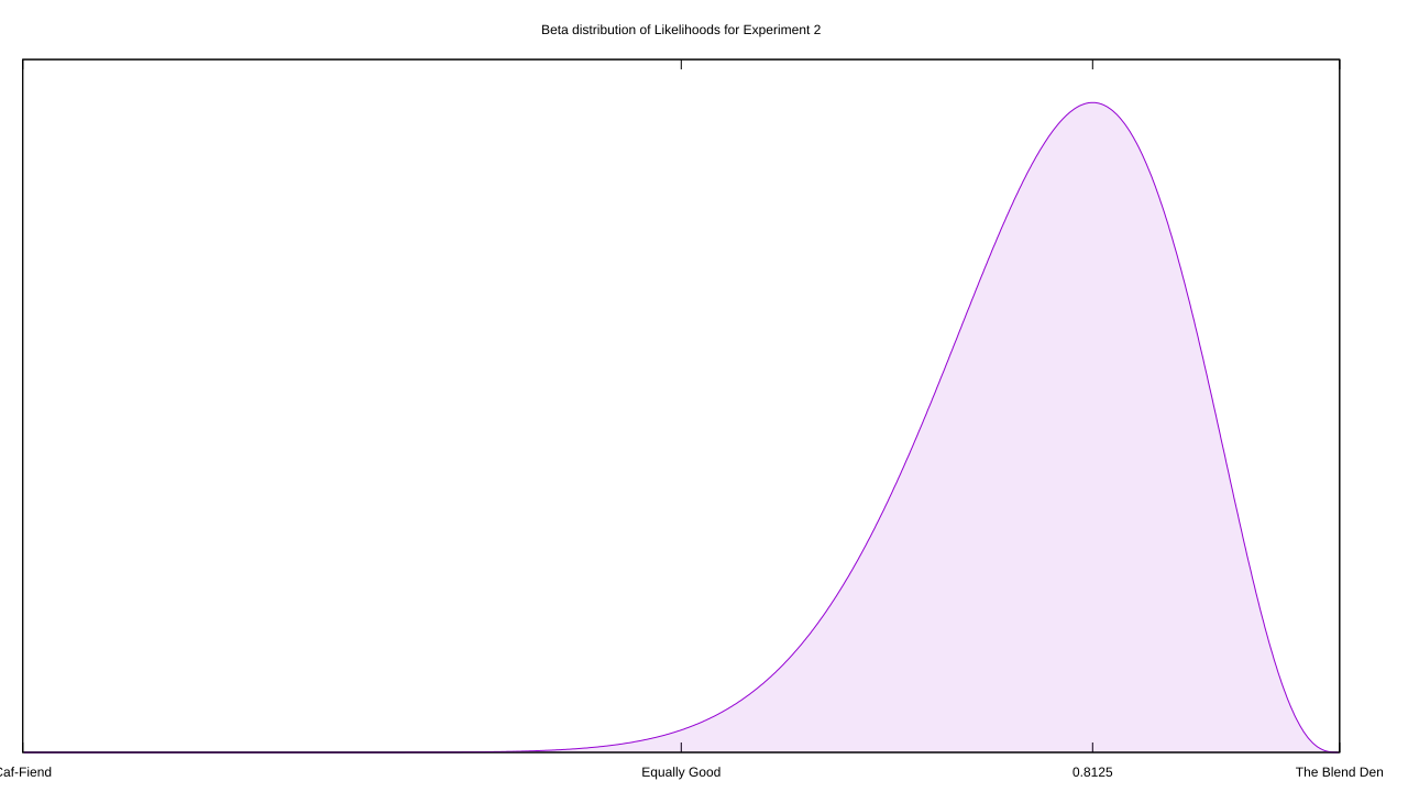
How do we use this distribution? I was tempted to build up a likelihood distributions for each hypothesis, but that’s equivalent to assigning probabilities to hypotheses and a no-no within frequentism. Instead, I can use another Beta distribution as an anchor: I feed it an equivalent amount of evidence, but split equally between Caf-Fiend and The Blend Den, then figure out where 95% of that distribution lies. I convert those bounds into a test statistic.
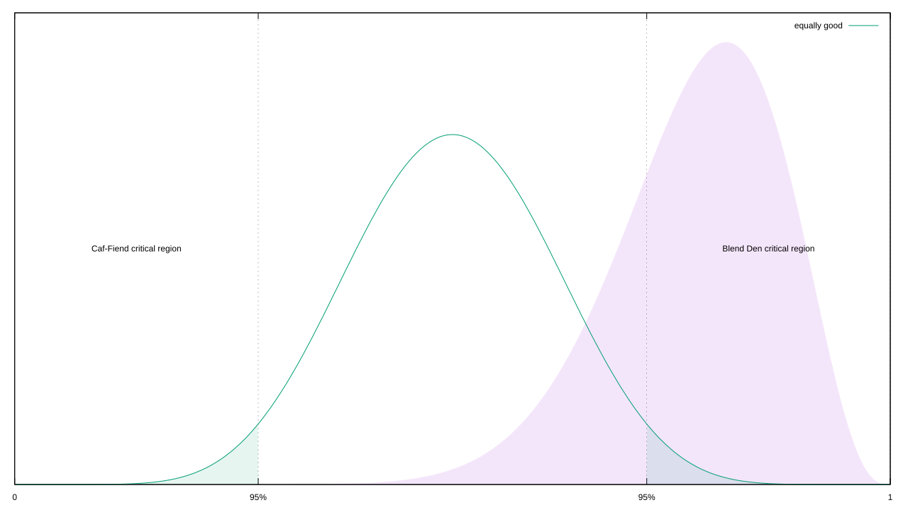
Now we can proceed with a frequentist analysis. The Fisher branch would integrate the area outside of The Blend Den’s critical region, and check if it’s less than 0.05; plug some magic words into Wolfram Alpha, and we find it’s nearer to 0.261546, so we fail to reject.
The Neyman-Pearson branch would find the maximum likelihood in each of these three regions and compare likelihood ratios; for Caf-Fiend, that’s at roughly x = 0.278118, for the equality hypothesis that’s x = 0.721882, and Blend Den peaks at x = 0.8125. In this case, a threshold of 1/20 is more appropriate than 1/19, because we’re not dealing with mutually-exclusive hypotheses. The theory that The Blend Den is better than Caf-Fiend easily hits that target (Likelihood Ratio ~= 0.0000505), but it doesn’t reject when matched with both coffee houses being equally as good (~0.7015).
Notice that we’ve coming to slightly different conclusions than the episode, which used paired t-tests to calculate a p-value of 0.005823 for The Blend Den having superior coffee. For that matter, Fisherian and Neyman-Pearson-style frequentism come to slightly different conclusions too!
That’s a rather important point, actually. One objection to Bayesian statistics is that it’s subjective; depending on the method you choose and evidence you include, different people can come to different outcomes. By focusing on long-term behaviour and falsifiability, frequentism is supposed to be much more objective and universal. Yet we’ve also reached different conclusions within frequentism!
In reality, frequentism is no less subjective than Bayesian statistics, the two only differ in where that subjectivity appears. With Bayes it’s right up front in big bold letters, via your choice of likelihood and prior; with frequentism, it’s hidden in the statistical distribution and methodology. That episode on t-tests assumed the data was best described by the Gaussian distribution. When I instead used the Beta or Binomial, their more diffuse spread of likelihood led to different conclusions. When I assumed the truthhood of a hypothesis depends only on the data, as in Fisherian frequentism, I got different results then when I assumed that truthhood was also dependent on how likely other hypotheses were.
I’m not mad or even disappointed in Hill and Crash Course; these blind spots are a structural part of frequentism. Since it’s portrayed as “objective,” even experienced pros can fail to recognise the assumptions they’ve made, let alone how those can distort their conclusions. In short, there is no free ticket to heaven for frequentists.