Gaining Credibility

You might have wondered why I didn’t pair my frequentist analysis in this post with a Bayesian one. Two reasons: length, and quite honestly I needed some time to chew over hypotheses. The default frequentist ones are entirely inadequate, for starters:

  • null: The data follows a Gaussian distribution with a mean of zero.
  • alternative: The data follows a Gaussian distribution with a non-zero mean.

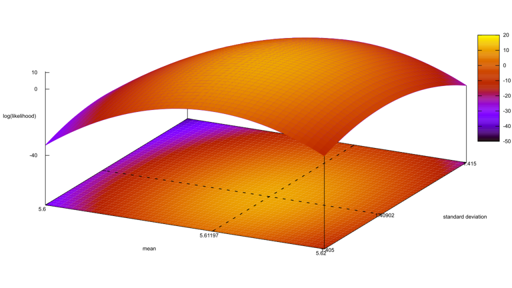
In chart form, their relative likelihoods look like this. [Read more…]

Continued Fractions

If you’ve followed my work for a while, you’ve probably noted my love of low-discrepancy sequences. Any time I want to do a uniform sample, and I’m not sure when I’ll stop, I’ll reach for an additive recurrence: repeatedly sum an irrational number with itself, check if the sum is bigger than one, and if so chop it down. Dirt easy, super-fast, and most of the time it gives great results.

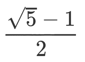
But finding the best irrational numbers to add has been a bit of a juggle. The Wikipedia page recommends primes, but it also claimed this was the best choice of all:\frac{\sqrt{5} - 1}{2}

I couldn’t see why. I made a half-hearted attempt at digging through the references, but it got too complicated for me and I was more focused on the results, anyway. So I quickly shelved that and returned to just trusting that they worked.

That is, until this Numberphile video explained them with crystal clarity. Not getting the connection? The worst possible number to use in an additive recurrence is a rational number: it’ll start repeating earlier points and you’ll miss at least half the numbers you could have used. This is precisely like having outward spokes on your flower (no seriously, watch the video), and so you’re also looking for any irrational number that’s poorly approximated by any rational number. And, wouldn’t you know it…

\frac{\sqrt{5} - 1}{2} ~=~ \frac{\sqrt{5} + 1}{2} - 1 ~=~ \phi - 1

… I’ve relied on the Golden Ratio without realising it.

Want to play around a bit with continued fractions? I whipped up a bit of Go which allows you to translate any number into the integer sequence behind its fraction. Go ahead, muck with the thing and see what patterns pop out.

Abductive and Inferential Science

I love it when Professor Moriarty wanders back to YouTube, and his latest was pretty good. He got into a spot of trouble at the end, which led me to muse on writing a blog post to help him out. I’ve already covered some of that territory, alas, but in the process I also stumbled on something more interesting to blog about. It also effects Sean Carroll’s paper, which Moriarty relied on.

The fulcrum of my topic is the distinction between inference and abduction. The former goes “I have a hypothesis, what does the data say about it?,” while the latter goes “I have data, can I find a hypothesis which explains it?” Moriarty uses this as a refutation of falsification: if we start from the data instead of the hypothesis, we’re not trying to falsify anything! To add salt to the wound, Moriarty argues (and I agree) that a majority of scientific activity consists of abduction and not inference; it’s quite common for scientists to jump from one topic to another, essentially engaging in a tonne of abductive activity until someone forces them to write up a hypothesis. Sean Carroll doesn’t dwell on this as much, but his paper does treat abduction and inference as separate things.

They aren’t separate, at least when it comes to the Bayesian interpretation of statistics. Let’s use a toy example to explain how; here’s a black box with a clear cover:

import ("math/rand")

func blackbox() float64 {

     x := rand.Float64()
     return (4111 + x*(4619 + x*(3627 + x*(7392*x - 9206)))/1213
     }

Each time we turn the crank on this function, we get back a number of some sort. The abductive way to analyse this is pretty straightforward: we grab a tonne of numbers and look for a hypothesis. I’ll go for the mean, median, and standard deviation here, the minimum I’ll need to check for a Gaussian distribution.

Samples = 1000001
Mean    = 5.61148
Std.Dev = 1.40887
Median  = 5.47287

Looks like there’s a slight skew downwards, but it’s not that bad. So I’ll propose that the output of this black box follows a Gaussian distribution, with mean 5.612 and standard deviation 1.409, until I can think of a better hypothesis which handles the skew.

After we reset for the inferential analysis, we immediately run into a problem: this is a black box. We know it has no input, and outputs a floating-point number, and that’s it. How can we form any hypothesis, let alone a null and alternative? We’ve no choice but to make something up. I’ll set my null to be “the black box outputs a random floating-point number,” and the alternative to “the output follows a Gaussian distribution with a mean of 0 and a standard deviation of 1.” Turn the crank, aaaand…

Samples            = 1000001
log(Bayes Factor)  = 26705438.01142
  (That means the most likely hypothesis is H1 (Gaussian distribution, mean = 0, std.dev = 1))

Unsurprisingly, our alternative does a lot better than our null. But our alternative is wrong! We’d get that impression pretty quickly if we watched the numbers streaming in. There’s an incredible temptation to take that data to refine or propose a new hypothesis, but that’s an abductive move. Inference is really letting us down.

Worse, this black box isn’t too far off from the typical science experiment. It’s rare any researcher is querying a black box, true, but it’s overwhelmingly true that they’re generating new data without incorporating other people’s datasets. It’s also rare you’re replicating someone else’s work; most likely, you’re taking existing ideas and rearranging them into something new, so prior findings may not carry forward. Inferential analysis is more tractable than I painted it, I’ll confess, but the limited information and focus on novelty still favors the abductive approach.

But think a bit about what I did on the inferential side: I picked two hypotheses and pitted them against one another. Do I have to limit myself to two? Certainly not! Let’s rerun the analysis with twenty-two hypotheses: the flat distribution we used as a null before, plus twenty-one alternative hypotheses covering every integral mean from -10 to 10 (though keeping the standard deviation at 1).

Samples                                 = 100001
log(likelihood*prior), H0               = -4436161.89971
log(likelihood*prior), H1, mean = -10   = -12378220.82173
log(likelihood*prior), H1, mean =  -9   = -10866965.39358
log(likelihood*prior), H1, mean =  -8   = -9455710.96544
log(likelihood*prior), H1, mean =  -7   = -8144457.53730
log(likelihood*prior), H1, mean =  -6   = -6933205.10915
log(likelihood*prior), H1, mean =  -5   = -5821953.68101
log(likelihood*prior), H1, mean =  -4   = -4810703.25287
log(likelihood*prior), H1, mean =  -3   = -3899453.82472
log(likelihood*prior), H1, mean =  -2   = -3088205.39658
log(likelihood*prior), H1, mean =  -1   = -2376957.96844
log(likelihood*prior), H1, mean =   0   = -1765711.54029
log(likelihood*prior), H1, mean =   1   = -1254466.11215
log(likelihood*prior), H1, mean =   2   = -843221.68401
log(likelihood*prior), H1, mean =   3   = -531978.25586
log(likelihood*prior), H1, mean =   4   = -320735.82772
log(likelihood*prior), H1, mean =   5   = -209494.39958
log(likelihood*prior), H1, mean =   6   = -198253.97143
log(likelihood*prior), H1, mean =   7   = -287014.54329
log(likelihood*prior), H1, mean =   8   = -475776.11515
log(likelihood*prior), H1, mean =   9   = -764538.68700
log(likelihood*prior), H1, mean =  10   = -1153302.25886
  (That means the most likely hypothesis is H1 (Gaussian distribution, mean = 6, std.dev = 1))

Aha, the inferential approach has finally gotten us somewhere! It’s still wrong, but you can see the obvious solution: come up with as many hypotheses as you can to explain the data, before we look at it, and run them all as the data rolls in. If you’re worried about being swamped by hypotheses, I’ve got a word for you: marginalization. Bayesian statistics handles hypotheses with parameters by integrating over all of them; you can think of these as composites, a mash of point hypotheses which collectively do a helluva lot better at prediction than any one hypothesis in isolation. In practice, then, Bayesians have always dealt with large numbers of hypotheses simultaneously.

The classic example of this is conjugate priors, where we carefully combine hyperparameters to evaluate a potentially infinite family of probability distributions. In fact, let’s try it right now: the proper conjugate here is the Normal-Inverse-Gamma, as we’re tracking both the mean and standard deviation of Gaussian distributions.

Samples = 1000001
μ       = 5.61148
λ       = 1000001.00000
α       = 500000.50000
β       = 992457.82655

median  = 5.47287

That’s a good start, μ lines up with the mean we calculated earlier, and λ is obviously the sample count. The shape of the posteriors is still pretty opaque, though; we’ll need to chart this out by evaluating the Normal-Inverse-Gamma PDF a few times.Conjugate posterior for the collection of all Gaussian distributions which could describe the data.Excellent, the inferential method has caught up to abduction! In fact, as of now they’re both working identically. Think: what’s the difference between a hypothesis you proposed before collecting the data, and one you proposed after? In frequentism, the stopping problem implies that we could exit early and falsely reject our null, when data coming down the pipe would have pushed it back to “fail to reject.” There, the choice of hypothesis could have an influence on the outcome, so there is a difference between the two cases. This is made worse by frequentism’s obsession over one hypothesis above all others, the null.

Bayesian statistics is free of that problem, because every hypothesis is judged on their relative likelihood in reference to a dataset shared by all hypotheses. There is no stopping problem baked into the methodology. Whether I evaluate any given hypothesis before or after I collect the data is irrelevant, because either way it has to cope with all the data. This also frees me up to invent hypotheses whenever I wish.

But this also defeats the main attack against falsification. The whole point of invoking abduction was to save us from asserting any hypotheses in the beginning; if there’s no difference in when we invoke our hypotheses, however, then falsification might still apply.

Here’s where I return to giving Professor Moriarity a hand. He began that video by saying scientists usually don’t engage in falsification, hence it cannot be The Scientific Method, but ended it by approvingly quoting Feynman: “We are trying to prove ourselves wrong as quickly as possible, because only in that way can we find progress.” Isn’t that falsification, right there?

This is yet another area where frequentist and Bayesian statistics diverge. As I pointed out earlier, frequentism is obsessed with falsifying the null hypothesis and trying to prove it wrong. Compare and contrast with what past-me wrote about Bayes Factors:

If data comes up that doesn’t square well with a hypothesis, its certainty takes a hit. But if we’re comparing it to another hypothesis that also doesn’t predict the data, the Bayes Factor will remain close to 1 and our certainties won’t shift much at all. Likewise, if both hypotheses strongly predict the data, the Factor again stays close to 1. If we’re looking to really shift our certainty around, we need a big Bayes Factor, which means we need to find scenarios where one hypothesis strongly predicts the data while the other strongly predicts this data shouldn’t happen.

Or, in other words, we should look for situations where one theory is… false. That sounds an awful lot like falsification!

But it’s not the same thing. Scroll back up to that Normal-Inverse-Gamma PDF, and pick a random point on the graph. The likelihood at that point is less than the likelihood at the maximum point. If you were watching those two points as we updated with new data, your choice would have gradually gone from about equally likely to substantially less likely. Your choice is more likely to be false, all things being equal, but it’s also not false with a capital F. Maybe the first million data points were a fluke, and if we continued sampling to a billion your choice would roar back to the top? This is the flip-side of having no stopping problem: the door is always left open a crack for any crackpot hypotheses to make a comeback.

Now look closely at the scale of the vertical axis. That maximal likelihood is well above 100%! In fact it’s somewhere around 4,023,000% by my calculations. While the vast majority are dropping downwards, there’s an ever-shrinking huddle of points that are becoming more likely as data is added! Falsification should only make things less likely, however.

Under Bayesian statistics, falsification is treated as a heuristic rather than a core part of the process. We’re best served by trying to find areas where hypotheses differ, yet we never declare one hypothesis to be false. This saves Moriarty: he’s both correct in disclaiming falsification, and endorsing the process of trying to prove yourself wrong. The confusion between the two stems from having to deal with two separate paradigms that appear to have substantial overlap, even though a closer look reveals fundamental differences.

Bayes’ Theorem: Deceptively Simple

Bayes' Theorem, in classic form

Good ol’ Bayes’ Theorem. Have you even wondered where it comes from, though? If you don’t know probability, there doesn’t seem to be any obvious logic to it. Once you’ve had it explained to you, though, it seems blindingly obvious and almost tautological. I know of a couple of good explainers, such as E.T. Jaynes’ Probability Theory, but just for fun I challenged myself to re-derive the Theorem from scratch. Took me about twenty minutes; if you’d like to try, stop reading here and try working it out yourself.

[Read more…]

Women’s Work

[I know, I’m a good three months late on this. It’s too good for the trash bin, though, and knowing CompSci it’ll be relevant again within the next year.]

This swells my heart.

LAURIE SEGALL: Computer science, it hasn’t always been dominated by men. It wasn’t until 1984 that the number of women studying computer science started falling. So how does that fit into your argument as to why there aren’t more women in tech?

JAMES DAMORE: So there are several reasons for why it was like that. Partly, women weren’t allowed to work other jobs so there was less freedom for people; and, also… it was simply different kinds of work. It was more like accounting rather than modern-day computer programming. And it wasn’t as lucrative, so part of the reason so many men give go into tech is because it’s high paying. I know of many people at Google that- they weren’t necessarily passionate about it, but it was what would provide for their family, and so they still worked there.

SEGALL: You say those jobs are more like accounting. I mean, look at Grace Hopper who pioneered computer programming; Margaret Hamilton, who created the first ever software which was responsible for landing humans on the moon; Katherine Johnson, Mary Jackson, Dorothy Vaughan, they were responsible for John Glenn accurately making his trajectory to the moon. Those aren’t accounting-type jobs?

DAMORE: Yeah, so, there were select positions that weren’t, and women are definitely capable of being confident programmers.

SEGALL: Do you believe those women were outliers?

DAMORE: … No, I’m just saying that there are confident women programmers. There are many at Google, and the women at Google aren’t any worse than the men at Google.

Segall deserves kudos for getting Damore to reverse himself. Even he admits there’s no evidence women are worse coders than men, in line with the current scientific evidence. I’m also fond of the people who make solid logical arguments against Damore’s views. We even have good research on why computing went from being dominated by women to dominated by men, and how occupations flip between male- and female-dominated as their social standing changes.

But there’s something lacking in Segall’s presentation of the history of women in computing. She isn’t alone, I’ve been reading a tonne of stories about the history of women in computing, and all of them suffer from the same omission: why did women dominate computing, at first? We think of math and logic as being “a guy thing,” so this is terribly strange. [Read more…]

Stochastic Supertasks

I really loved this illustration of the paradoxes of infinity from Infinite Series, so much so that I’ll sum it up here.

What if you could do one task an infinite number of times over a finite time span? The obvious thing to do, granted this superpower, is start depositing money into your bank account. Let’s say you decide on plunking in one dollar at a time, an infinite number of times. Not happy at having to process an infinite number of transactions, your bank decides to withdraw a 1 cent fee after every one. How much money do you have in your bank account, once the dust settles?

Zero bucks. Think about it: at some point during the task you’ll have deposited N dollars in the account. The total amount the bank takes, however, keeps growing over time and at some point it’s guaranteed to reach N dollars too. This works for any value of N, and so any amount of cash you deposit will get removed.

In contrast, if the bank had decided to knock off 1 cent of your deposit before it reached your bank account, you’d both have an infinite amount of cash! This time around, there is no explicit subtraction to balance against the deposits, so your funds grow without bounds.

Weird, right? Welcome to the Ross–Littlewood paradox. My formulation is a bit more fun than the original balls-and-urns approach, but does almost the same job (picture the balls as pennies). It does fail when it comes to removing a specific item from the container, though; in the Infinite Series video, the host challenges everyone to figure out what happens if you remove the median ball from the urn after adding nine, assuming each ball has a unique number assigned to it. Can’t do that with cash.

My attempt is below the fold.

[Read more…]

“Science Is Endangered by Statistical Misunderstanding”

He’s baaaaaack. I’ve linked to David Colquhoun’s previous paper on p-values,[1] but I’ve since learned he’s about to publish a sequel.

Despite decades of warnings, many areas of science still insist on labelling a result of P < 0.05 as “significant”.   This practice must account for a substantial part of the lack of reproducibility in some areas of science. And this is before you get to the many other well-known problems, like multiple comparisons, lack of randomisation and P-hacking. Science is endangered by statistical misunderstanding, and by university presidents and research funders who impose perverse incentives on scientists. [2]

[Read more…]

Math Can Be Weird

Take the Cantor function, a “Devil’s Staircase.”

The Cantor function, in the range [0:1]. It looks like a jagged staircase.

It looks like a squiggly mess, yet it is continuous and at almost every point there’s a well-defined slope: perfectly horizontal. The only exceptions are at points along the X-axis which are part of the Cantor set, an uncountable number of points with zero length. Even at one of these points, however, the net vertical increase is zero! We can see this by calculating the limits toward a point with a non-zero slope.

Wikipedia has a good write-up on how to evaluate the Cantor function (I used it in the above approximation).

  1. Express x in base 3.
  2. If x contains a 1, replace every digit after the first 1 by 0.
  3. Replace all 2s with 1s.
  4. Interpret the result as a binary number. The result is c(x).

The point x = 1/3 is part of the Cantor set, and thus satisfies our needs. Following the above rules, the output of the function there is 0.1 in binary, or 0.5 in decimal. Let’s calculate both limits, to get a feel for how much vertical is climbed at that point.

Approaching the limits of C(1/3). Spoiler alert, they both wind up equalling 1/2.

If we approach x = 1/3 from the right, we flatline at y = 1/2 . If  we approach it from the left, we wind up evaluating the geometric series y = 1/4 + 1/8 + 1/16 + … to calculate the height, which gets arbitrarily close to y = 1/2 . The height of the “jump” at x = 1/3 vanishes into insignificance! That’s a good thing, as otherwise the Cantor function’s slope would have approached a vertical line and it wouldn’t be a function.

Calculating the slope of the Cantor function at x = 1/3. Spoiler alert, it approaches a perfectly vertical slope.

Yet even though every single vertical hop is arbitrarily small, it’s obvious the Cantor function has some sort of vertical increase. How else could it contain both (0,0) and (1,1)?  In fact, if you measured the arc length of the Cantor function, it would be two units. Every point where the slope isn’t horizontal it is arbitrarily vertical, so no matter where you put the vertical or horizontal bits you wind up travelling the Manhattan distance between (0,0) and (1,1), which is 2. We know the distance of the horizontal components adds to one unit, since the Cantor set has length 0 and the horizontal distance is 1, so the uncountable number of arbitrarily small vertical “hops” must also have a net length of one unit.

The Cantor function manages to climb vertically without actually climbing vertically. Pretty wild, eh?

Oh, and credit where credit is due, I was introduced to the Cantor function by PBS’s Infinite Series. Check it out for a weekly dose of math.