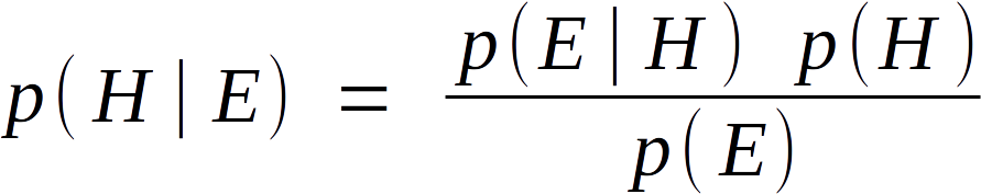
Good ol’ Bayes’ Theorem. Have you even wondered where it comes from, though? If you don’t know probability, there doesn’t seem to be any obvious logic to it. Once you’ve had it explained to you, though, it seems blindingly obvious and almost tautological. I know of a couple of good explainers, such as E.T. Jaynes’ Probability Theory, but just for fun I challenged myself to re-derive the Theorem from scratch. Took me about twenty minutes; if you’d like to try, stop reading here and try working it out yourself.
Right, let’s start with a Venn diagram.
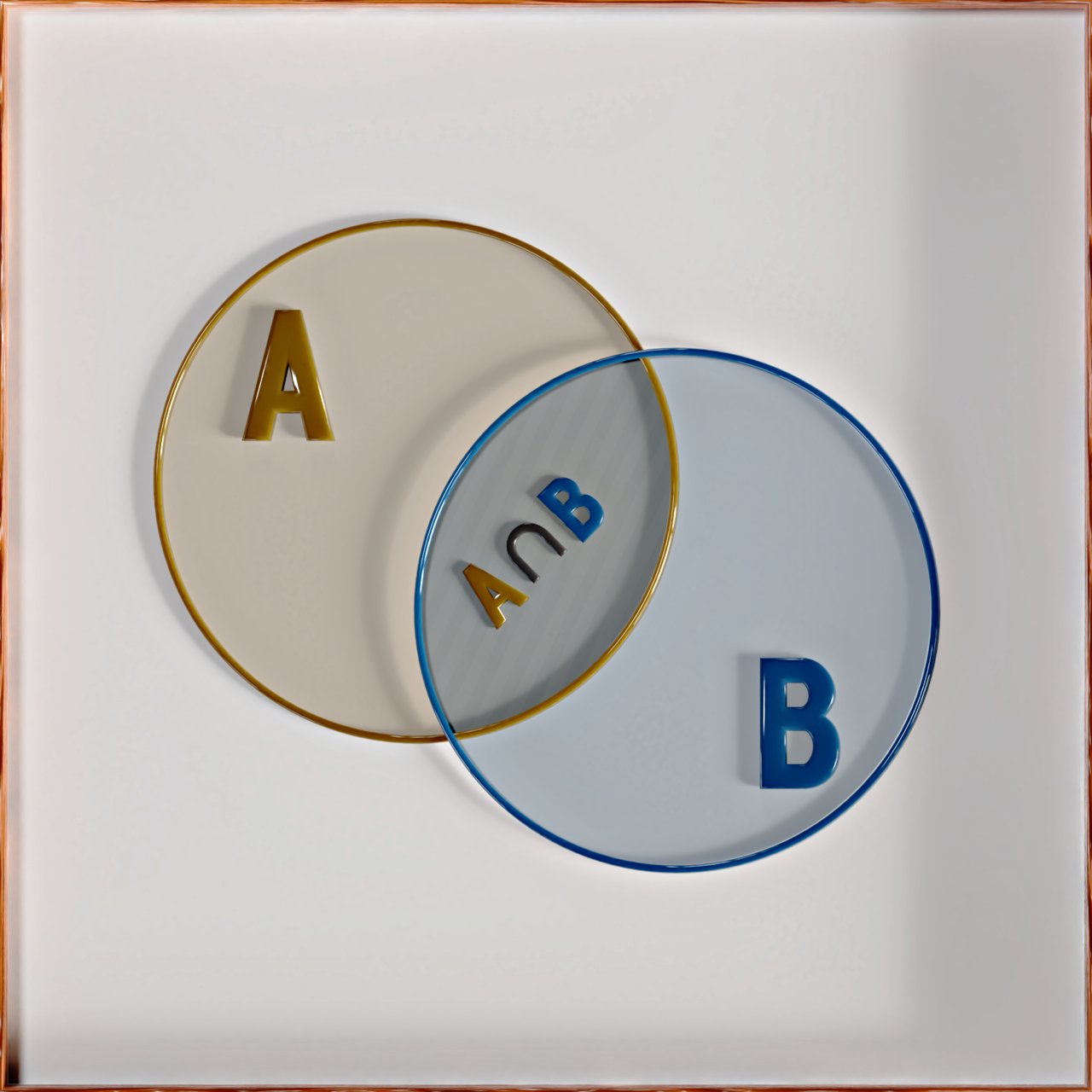
This entire square represents everything we care about here. “A” is one section of this universe, “B” is another, and the two of them might overlap to some degree. The only assumptions were making here are that the size of A, written as “|A|,” is greater than zero, as is |B| or the size of B, and that both A and B fit entirely within the universe. We’re not saying anything else about the size of those sections, or how much they overlap. That section can be written as A ∩ B, or “the intersection of A and B.”
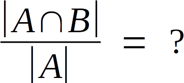
Let’s say we’re interested in the relative sizes between two sections of this chart. Specifically, we want to calculate this:
We can start by doing a basic math trick. If you multiply something by a number that isn’t zero, then divide by that number again, you get back the original number you started with. So let’s invoke that with the value of |B|.
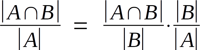
This seems to be moving backwards, but it’ll come in handy once we finish talking about probabilities.
The easiest way to think of probability is the ratio of desired outcomes to possible outcomes. How would we calculate the probability of rolling a five on a die? Well, there’s one desired outcome (we roll the five), as well as six possible outcomes (we roll a one, two, three, and so on). One divided by six is 1/6. Pretty intuitive, right? So let’s turn the diagram above into a dartboard.
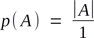
Suppose we randomly pick a spot above this board, and drop a dart onto it. What is the probability it would hit A? The area of A is |A|, so there are |A| desired outcomes here. To make the math easy, we’ll scale everything so the board has an area of one unit. Thus we can write that probability as
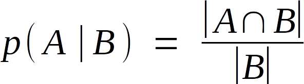
The same logic applies to p(B), of course. Let’s try something a bit trickier: let’s say we’ve dropped the dart and it hit B. What are the odds that it also happened to hit A? The mathematical shorthand for that question is “p( A | B ).” We know the number of possible outcomes here, |B|, and the desired outcomes happen in the area where A intersects B, so the answer is
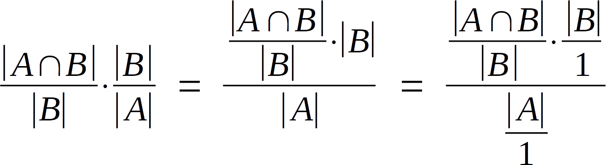
A-ha! We can repeat this logic for p( B | A ), too, then shuffle around that mysterious first equation a bit. For instance, the way the equation was set up implied we must divide |B| by |A| before multiplying by the left-hand fraction. Because we’re only doing multiplication and division, though, we can instead multiply first then divide by |A| later on. Dividing a number by one doesn’t change it, right? So we can pop those divisions in anywhere we find convenient. Applying all these tricks, we get
I think you can see where I’m going with this. By substituting in the probability expressions from above, we arrive at:
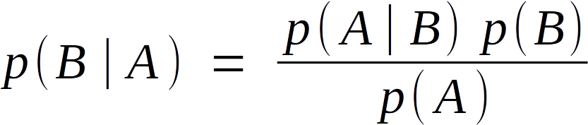
And from there we just need to state “B = H” and “A = E” to arrive back at Bayes’ Theorem. This makes it obvious why Bayesian statistics was once called “Inverse Probability,” as it permits you to calculate p( H | E ) from p( E | H ) and vice-versa.
I’ll admit there are much simpler derivations out there, but all the ones I’ve read fail to explain an obvious consequence. Recently, judges have rejected the use of Bayes’ Theorem in the courtroom. Ronald Fisher, who probably did more to bury Bayesian statistics than anyone else, nonetheless did everything he could to rescue the Reverend from his own Theorem.[1]
It has become realized in recent years (Fisher, 1958) that although Bayes considered the special axiom associated with his name for assigning probabilities a priori, and devoted a scholium to its discussion, in his actual mathematics he avoided this axiomatic approach as open to dispute, but showed that its purpose could be served by an auxiliary experiment, so that the probability statements a posteriori at which he arrived were freed from any reliance on the axiom, and shown to be demonstrable on the basis of observations only, such as are the source of new knowledge in the natural sciences.[2]
If Bayes’ Theorem is so trivial to derive, how can people reject it? Why did statistical giants like Fisher twist themselves in knots to avoid it?
One reason is that it has deep epistemological consequences. Think of a person, then ask yourself whether they have read this sentence. Either they have or they have not, and yet Bayes’ Theorem can attach numbers like 25% or 65.37% to it. How can someone 25% read that sentence? These numbers cannot represent actual things in the world, which is weird because when deriving Bayes’ Theorem I invoked counting.
The other reason is that I’m treating hypotheses and data as if they were the same thing. “Person X read that sentence” and “I observed person X reading that sentence” seem to be qualitatively different statements; the former is a potential truth about the world, the latter a sensation derived from direct interaction with the world. Yet according to our derivation they can be smushed together and measured using the same metric. Substituting H for B and E for A was a mere label switch. Under this interpretation, I can also write:

“The probability of seeing some evidence, dependent on the probability of seeing other evidence” seems non-controversial, but how can the probability of one hypothesis depend on another? What does “depend” even mean for something abstract and non-causal?
We can resolve these contradictions by denying that hypotheses carry a probability. Stating any part of the Venn diagram represents a hypothesis becomes a bogus move, though the rest of the logic behind Bayes’ Theorem remains legit. This is a core assumption of frequentist statistics.
For example, if I toss a coin, the probability of heads coming up is the proportion of times it produces heads. But it cannot be the proportion of times it produces heads in any finite number of tosses. If I toss the coin 10 times and it lands heads 7 times, the probability of a head is not therefore 0.7. A fair coin could easily produce 7 heads in 10 tosses. The relative frequency must refer therefore to a hypothetical infinite number of tosses. The hypothetical infinite set of tosses (or events, more generally) is called the reference class or collective. […]
[In another experiment,] Each event is ‘throwing a fair die 25 times and observing the number of threes’. That is one event. Consider a hypothetical collective of an infinite number of such events. We can then determine the proportion of such events in which the number of threes is 5. That is a meaningful probability we can calculate. However, we cannot talk about P(H | D), for example P(‘I have a fair die’ | ‘I obtained 5 threes in 25 rolls’), [or] the probability that the hypothesis that I have a fair die is true, given I obtained 5 threes in 25 rolls. What is the collective? There is none. The hypothesis is simply true or false. [3]
We are inclined to think that as far as a particular hypothesis is concerned, no test based upon the theory of probability can by itself provide any valuable evidence of the truth or falsehood of that hypothesis.[4]
This answer is not perfect. A minor complaint is that most probability systems have values that can represent “absolutely true” and “absolutely false,” so there’s no obvious theoretical barrier to including hypotheses.
More importantly, consider the first example of Eliezer S. Yudkowsky’s famous introduction to Bayes’ Theorem.
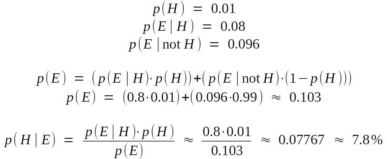
1% of women at age forty who participate in routine screening have breast cancer. 80% of women with breast cancer will get positive mammographies. 9.6% of women without breast cancer will also get positive mammographies. A woman in this age group had a positive mammography in a routine screening. What is the probability that she actually has breast cancer?
Out of 10,000 women, 100 have breast cancer; 80 of those 100 have positive mammographies. From the same 10,000 women, 9,900 will not have breast cancer and of those 9,900 women, 950 will also get positive mammographies. This makes the total number of women with positive mammographies 950+80 or 1,030. Of those 1,030 women with positive mammographies, 80 will have cancer. Expressed as a proportion, this is 80/1,030 or 0.07767 or 7.8%.
[1] Aldrich, John. “RA Fisher on Bayes and Bayes’ theorem.” Bayesian Analysis 3.1 (2008): 161-170.
[2] Fisher, Ronald. “Some examples of Bayes’ method of the experimental determination of probabilities a priori.” Journal of the Royal Statistical Society. Series B (Methodological)(1962): 118-124.
[3] Dienes, Zoltan. Understanding Psychology as a Science: An Introduction to Scientific and Statistical Inference. Palgrave Macmillan, 2008. pg. 58-59
[4] Neyman, Jerzy, and Egon S. Pearson. On the Problem of the Most Efficient Tests of Statistical Hypotheses. Springer, 1933. http://link.springer.com/chapter/10.1007/978-1-4612-0919-5_6.