I still can’t believe this post exists, given its humble beginnings.
The “women’s category” is, in my opinion, poorly named given our current climate, and so I’d elect a name more along the lines of the “Under 5 nmol/l category” (as in, under 5 nanomoles of testosterone per litre), but make no mistake about it, the “woman’s category” is not based on gender or identity, or even genitalia or chromosomes… it’s based on hormone levels and the absence of male puberty.
The above comment wasn’t in Rationality Rules’ latest transphobic video, it was just a casual aside by RR himself in the YouTube comment section. He’s obiquely doubled-down via Twitter (hat tip to Essence of Thought):
Of course, just as I support trans men competing in all “men’s categories” (poorly named), women who have not experienced male puberty competing in all women’s sport (also poorly named) and trans women who have experienced male puberty competing in long-distance running.
To further clarify, I think that we must rename our categories according to what they’re actually based on. It’s not right to have a “women’s category” and yet say to some trans women (who are women!) that they can’t compete within it; it should be renamed.
The proposal itched away at me, though, because I knew it was testable.
There is a need to clarify hormone profiles that may be expected to occur after competition when antidoping tests are usually made. In this study, we report on the hormonal profile of 693 elite athletes, sampled within 2 h of a national or international competitive event. These elite athletes are a subset of the cross-sectional study that was a component of the GH-2000 research project aimed at developing a test to detect abuse with growth hormone.
Healy, Marie-Louise, et al. “Endocrine profiles in 693 elite athletes in the postcompetition setting.” Clinical endocrinology 81.2 (2014): 294-305.
The GH-2000 project had already done the hard work of collecting and analyzing blood samples from athletes, so checking RR’s proposal was no tougher than running some numbers. There’s all sorts of ethical guidelines around sharing medical info, but fortunately there’s an easy shortcut: ask one of the scientists involved to run the numbers for me, and report back the results. Aggregate data is much more resistant to de-anonymization, so the ethical concerns are greatly reduced. The catch, of course, is that I’d have to find a friendly researcher with access to that dataset. About a month ago, I fired off some emails and hoped for the best.
I wound up much, much better than the best. I got full access to the dataset!! You don’t get handed an incredible gift like this and merely use it for a blog post. In my spare time, I’m flexing my Bayesian muscles to do a re-analysis of the above paper, while also looking for observations the original authors may have missed. Alas, that means my slow posting schedule is about to crawl.
But in the meantime, we have a question to answer.
What Do We Have Here? 
Total Assigned-female Athletes = 239
  Height, Mean           = 171.61 cm
  Height, Std.Dev        = 7.12 cm
  Weight, Mean           = 64.27 kg
  Weight, Std.Dev        = 9.12 kg
  Body Fat, Mean         = 13.19 kg
  Body Fat, Std.Dev      = 3.85 kg
  Testosterone, Mean     = 2.68 nmol/L
  Testosterone, Std.Dev  = 4.33 nmol/L
  Testosterone, Max      = 31.90 nmol/L
  Testosterone, Min      = 0.00 nmol/L

Total Assigned-male Athletes = 454
  Height, Mean           = 182.72 cm
  Height, Std.Dev        = 8.48 cm
  Weight, Mean           = 80.65 kg
  Weight, Std.Dev        = 12.62 kg
  Body Fat, Mean         = 8.89 kg
  Body Fat, Std.Dev      = 7.20 kg
  Testosterone, Mean     = 14.59 nmol/L
  Testosterone, Std.Dev  = 6.66 nmol/L
  Testosterone, Max      = 41.00 nmol/L
  Testosterone, Min      = 0.80 nmol/L
The first step is to get a basic grasp on what’s there, via some crude descriptive statistics. It’s also useful to compare these with the original paper, to make sure I’m interpreting the data correctly. Excusing some minor differences in rounding, the above numbers match the paper.
The only thing that stands out from the above, to me, is the serum levels of testosterone. At least one source says the mean of these assigned-female athletes is higher than the normal range for their non-athletic cohorts. Part of that may simply be because we don’t have a good idea of what the normal range is, so it’s not uncommon for each lab to have their own definition of “normal.” This is even worse for those assigned female, since their testosterone levels are poorly studied; note that my previous link collected the data of over a million “men,” but doesn’t mention “women” once. Factor in inaccurate test results and other complicating factors, and “normal” is quite poorly-defined.
Still, Rationality Rules is either convinced those complications are irrelevant, or ignorant of them. And, to be fair, that 5nmol/L line implicitly sweeps a lot of them under the rug. Let’s carry on, then, and look for invalid data. “Invalid” covers everything from missing data, to impossible data, and maybe even data we think might be made inaccurate due to measurement error. I consider a concentration of zero testosterone as invalid, even though it may technically be possible.
Total Assigned-male Athletes w/ T levels >= 0        = 446
                             w/ T levels <= 0.5      = 0
                             w/ T levels == 0        = 0
                             w/ missing T levels     = 8
                             that I consider valid   = 446

Total Assigned-female Athletes w/ T levels >= 0      = 234
                               w/ T levels <= 0.5    = 5
                               w/ T levels == 0      = 1
                               w/ missing T levels   = 5
                               that I consider valid = 229
Fortunately for us, the losses are pretty small. 229 datapoints is a healthy sample size, so we can afford to be liberal about what we toss out. Next up, it would be handy to see the data in chart form.
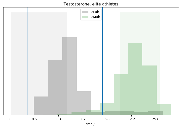
I've put vertical lines at both the 0.5 and 5 nmol/L cutoffs. There's a big difference between categories, but we can see clouds on the horizon: a substantial number of assigned-female athletes have greater than 5 nmol/L of testosterone in their bloodstream, while a decent number of assigned-male athletes have less. How many?
Segregating Athletes by Testosterone
Concentration  aFab  aMab
   > 5nmol/L    19   417
   < 5nmol/L   210    26
   = 5nmol/L     0     3

8.3% of assigned-female athletes have > 5nmol/L
5.8% of assigned-male athletes have < 5nmol/L
4.4% of athletes with > 5nmol/L are assigned-female
11.0% of athletes with < 5nmol/L are assigned-male
Looks like anywhere from 6-8% of athletes have testosterone levels that cross Rationality Rules' line. For comparison, maybe 1-2% of the general public has some level of gender dysphoria, though estimating exact figures is hard in the face of widespread discrimination and poor sex-ed in schools. Even that number is misleading, as the number of transgender athletes is substantially lower than 1-2% of the athletic population. The share of transgender athletes is irrelevant to this dataset anyway, as it was collected between 1996 and 1999, when no sporting agency had policies that allowed transgender athletes to openly compete.
That 6-8%, in other words, is entirely cisgender. This echoes one of Essence Of Thought's arguments: RR's 5nmol/L policy has far more impact on cis athletes than trans athletes, which could have catastrophic side-effects. Could is the operative word, though, because as of now we don't know anything about these athletes. Do >5nmol/L assigned-female athletes have bodies more like >5nmol/L assigned-male athletes than <5nmol/L assigned-female athletes? If so, then there's no problem. Equivalent body types are competing against each other, and outcomes are as fair as could be reasonably expected.
What, then, counts as an "equivalent" body type when it comes to sport?
Newton's First Law of Athletics 
One reasonable measure of equivalence is height. It's one of the stronger sex differences, and height is also correlated with longer limbs and greater leverage. Whether that's relevant to sports is debatable, but height and correlated attributes dominate Rationality Rules' list.
[19:07] In some events - such as long-distance running, in which hemoglobin and slow-twitch muscle fibers are vital - I think there's a strong argument to say no, [transgender women who transitioned after puberty] don't have an unfair advantage, as the primary attributes are sufficiently mitigated. But in most events, and especially those in which height, width, hip size, limb length, muscle mass, and muscle fiber type are the primary attributes - such as weightlifting, sprinting, hammer throw, javelin, netball, boxing, karate, basketball, rugby, judo, rowing, hockey, and many more - my answer is yes, most do have an unfair advantage.
Fortunately for both of us, most athletes in the dataset have a "valid" height, which I define as being at least 30cm tall.
Out of 693 athletes, 678 have valid height data.
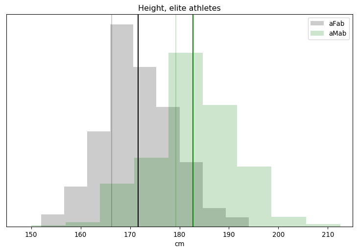
The faint vertical lines are for the mean adult height of Germans born in 1976, which should be a reasonable cohort to European athletes that were active between 1996 and 1999, while the darker lines are each category's mean. Athletes seem slightly taller than the reference average, but only by 2-5cm. The amount of overlap is also surprising, given that height is supposed to be a major sex difference. We actually saw less overlap with testosterone! Finally, the height distribution isn't quite Gaussian, there's a subtle bias towards the taller end of the spectrum.
Height is a pretty crude metric, though. You could pair any athlete with a non-athlete of the same height, and there's no way the latter would perform as well as the former. A better measure of sporting ability would be muscle mass. We shouldn't use the absolute mass, though: bigger bodies have more mass and need more force to accelerate as smaller bodies do, so height and muscle mass are correlated. We need some sort of dimensionless scaling factor which compensates.
And we have one! It's called the Body Mass Index, or BMI.
$$ BMI = \frac w {h^2}, $$
where \(w\) is a person's mass in kilograms, and \(h\) is a person's height in metres. Unfortunately, BMI is quite problematic. Partly that's because it is a crude measure of obesity. But part of that is because there are two types of tissue which can greatly vary, body fat and muscle, yet both contribute equally towards BMI.
That's all fixable. For one, some of the athletes in this dataset had their body fat measured. We can subtract that mass off, so their weight consists of tissues that are strongly correlated with height plus one that is fudgable: muscle mass. For two, we're not assessing these individual's health, we only want a dimensionless measure of muscle mass relative to height. For three, we're not comparing these individuals to the general public, so we're not restricted to using the general BMI formula. We can use something more accurate.
The oddity is the appearance of that exponent 2, though our world is three-dimensional. You might think that the exponent should simply be 3, but that doesn't match the data at all. It has been known for a long time that people don't scale in a perfectly linear fashion as they grow. I propose that a better approximation to the actual sizes and shapes of healthy bodies might be given by an exponent of 2.5. So here is the formula I think is worth considering as an alternative to the standard BMI:
$$ BMI' = 1.3 \frac w {h^{2.5}} $$
I can easily pop body fat into Nick Trefethen's formula, and get a better measure of relative muscle mass,
$$ \overline{BMI} = 1.3 \frac{ w - bf }{h^{2.5}}, $$
where \(bf\) is total body fat in kilograms. Individuals with excess muscle mass, relative to what we expect for their height, will have a high \(\overline{BMI}\), and vice-versa. And as we saw earlier, muscle mass is another of Rationality Rules' determinants of sporting performance.
Time for more number crunching.
Out of 693 athletes, 227 have valid adjusted BMIs.
                     663 have valid weights.
                     241 have valid body fat percentages.

Total Assigned-female Athletes = 239
 total with valid adjusted BMI = 86
  adjusted BMI, Mean     = 16.98
  adjusted BMI, Std.Dev  = 1.21
  adjusted BMI, Median   = 16.96

Total Assigned-male Athletes = 454
 total with valid adjusted BMI = 141
  adjusted BMI, Mean     = 20.56
  adjusted BMI, Std.Dev  = 1.88
  adjusted BMI, Median   = 20.28
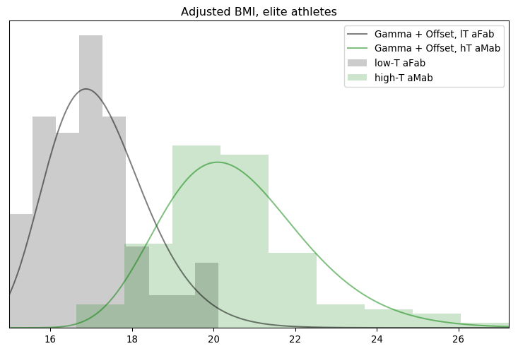
The bad news is that most of this dataset lacks any information on body fat, which really cuts into our sample size. The good news is that we've still got enough to carry on. It also looks like there's a strong sex difference, and the distribution is pretty clustered. Still, a chart would help clarify the latter point.
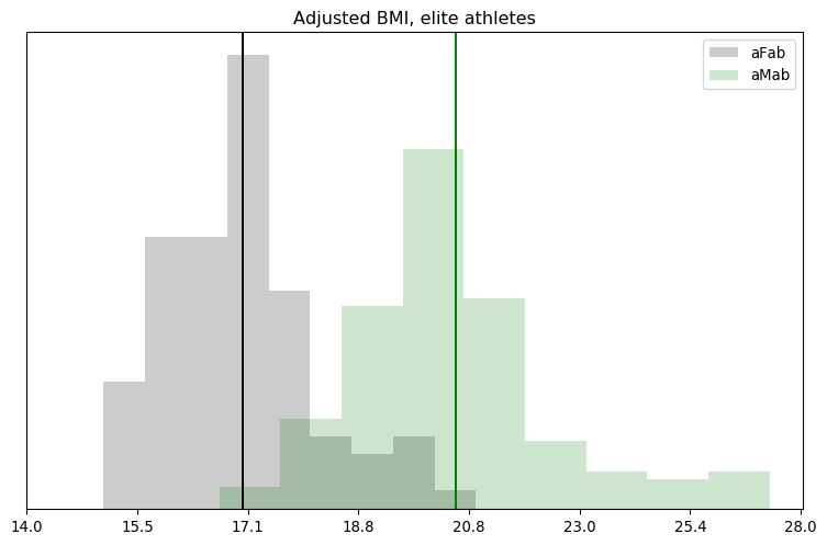
Whoops! There's more overlap and skew than I thought. Even in logspace, the results don't look Gaussian. We'll have to remember that for the next step.
A Man Without a Plan is Not a Man 
Just looking at charts isn't going to solve this question, we need to do some sort of hypothesis testing. Fortunately, all the pieces I need are here. We've got our hypothesis, for instance:
Athletes with exceptional testosterone levels are more like athletes of the same sex but with typical testosterone levels, than they are of other athletes with a different sex but similar testosterone levels.
If you know me, you know that I'm all about the Bayes, and that gives us our methodology.
- Fit a model to a specific metric for assigned-female athletes with less than 5nmol/L of serum testosterone.
- Fit a model to a specific metric for assigned-male athletes with more than 5nmol/L of serum testosterone.
- Apply the first model to the test group, calculating the overall likelihood.
- Apply the second model to the test group, calculating the overall likelihood.
- Sample the probability distribution of the Bayes Factor.
"Metric" is one of height or \(\overline{BMI}\), while "test group" is one of assigned-female athletes with >5nmol/L of serum testosterone or assigned-male athletes with <5nmol/L of serum testosterone. The Bayes Factor is simply
$$ \text{Bayes Factor} = \frac{ p(E \mid H_1) \cdot p(H_1) }{ p(E \mid H_2) \cdot p(H_2) } = \frac{ p(H_1 \mid E) }{ p(H_2 \mid E) }, $$
which means we need two hypotheses, not one. Fortunately, I've phrased the hypothesis to make it easy to negate: athletes with exceptional testosterone levels are less like athletes of the same sex but with typical testosterone levels, than they are of other athletes with a different sex but similar testosterone levels. We'll call this new hypothesis \(H_2\), and the original \(H_1\). Bayes factors greater than 1 mean \(H_1\) is more likely than \(H_2\), and vice-versa.
Calculating all that would be easy if I was using Stan or PyMC3, but I ran into problems translating the former's probability distributions into charts, and I don't have any experience with the latter. My next choice, emcee, forces me to manually convolve two posterior distributions. Annoying, but not difficult.
I'm a Model, If You Know What I Mean 
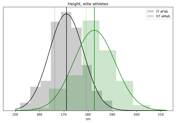
That just leaves one thing left: what models are we going to use? The obvious choice for height is the Gaussian distribution, as from previous research we know it's a great model.
Fitting the height of lT aFab athletes to a Gaussian distribution ...
     0: (-980.322471) mu=150.000819, sigma=15.000177
    64: (-710.417497) mu=169.639051, sigma=8.579088
   128: (-700.539260) mu=171.107358, sigma=7.138832
   192: (-700.535241) mu=171.154151, sigma=7.133279
   256: (-700.540692) mu=171.152701, sigma=7.145515
   320: (-700.552831) mu=171.139668, sigma=7.166857
   384: (-700.530969) mu=171.086422, sigma=7.094077
    ML: (-700.525284) mu=171.155240, sigma=7.085777
median: (-700.525487) mu=171.134614, sigma=7.070993
Alas, emcee also lacks a good way to assess model fitness. One crude metric is look at the progression of the mean fitness; if it grows and then stabilizes around a specific value, as it does here, we've converged on something. Another is to compare the mean, median, and maximal likelihood of the posterior; if they're about equally likely, we've got a fuzzy caterpillar. Again, that's also true here.
As we just saw, though, charts are a better judge of fitness than a handful of numbers.

If you were wondering why I didn't make much of a fuss out of the asymmetry in the height distribution, it's because I've already seen this graph. A good fit isn't necessarily the best though, and I might be able to get a closer match by incorporating the sport each athlete played.
            Assigned-female Athletes
         sport              below/above 171cm
           Power lifting:  1 / 0
              Basketball:  2 /12
                Football:  0 / 0
                Swimming: 41 /49
                Marathon:  0 / 1
                Canoeing:  1 / 0
                  Rowing:  9 /13
    Cross-country skiing:  8 / 1
           Alpine skiing: 11 / 1
          Weight lifting:  7 / 0
                    Judo:  0 / 0
                   Bandy:  0 / 0
              Ice Hockey:  0 / 0
                Handball: 12 /17
         Track and field: 22 /27
Basketball attracts tall people, unsurprisingly, while skiing seems to attract shorter people. This could be the cause of that asymmetry. It's no guarantee that I'll actually get a better fit, though, as I'm also dramatically cutting the number of datapoints to fit to. The model's uncertainty must increase as a result, and that may be enough to dilute out any increase in fitness. I'll run those numbers for the paper, but for now the Gaussian model I have is plenty good.
Fitting the height of hT aMab athletes to a Gaussian distribution ...
     0: (-2503.079578) mu=150.000061, sigma=15.001179
    64: (-1482.315571) mu=179.740851, sigma=10.506003
   128: (-1451.789027) mu=182.615810, sigma=8.620333
   192: (-1451.748336) mu=182.587979, sigma=8.550535
   256: (-1451.759883) mu=182.676004, sigma=8.546410
   320: (-1451.746697) mu=182.626918, sigma=8.538055
   384: (-1451.747266) mu=182.580692, sigma=8.534070
    ML: (-1451.746074) mu=182.591047, sigma=8.534584
median: (-1451.759295) mu=182.603231, sigma=8.481894
We get the same results when fitting the model to >5 nmol/L assigned-male athletes. The log likelihood, that number in brackets, is a lot lower for these athletes, but that number is roughly proportional to the number of samples. If we had the same degree of model fitness but doubled the number of samples, we'd expect the log likelihood to double. And, sure enough, this dataset has roughly twice as many assigned-male athletes as it does assigned-female athletes.
The updated charts are more of the same.
Unfortunately, adjusted BMI isn't nearly as tidy. I don't have any prior knowledge that would favour a particular model, so I wound up testing five candidates: the Gaussian, Log-Gaussian, Gamma, Weibull, and Rayleigh distributions. All but the first needed an offset parameter to get the best results, which has the same interpretation as last time.
Fitting the adjusted BMI of hT aMab athletes to a Gaussian distribution ...
     0: (-410.901047) mu=14.999563, sigma=5.000388
   384: (-256.474147) mu=20.443497, sigma=1.783979
    ML: (-256.461460) mu=20.452817, sigma=1.771653
median: (-256.477475) mu=20.427138, sigma=1.781139
Fitting the adjusted BMI of hT aMab athletes to a Log-Gaussian distribution ...
     0: (-629.141577) mu=6.999492, sigma=2.001107, off=10.000768
   384: (-290.910651) mu=3.812746, sigma=1.789607, off=16.633741
   ML: (-277.119315) mu=3.848383, sigma=1.818429, off=16.637382
median: (-288.278918) mu=3.795675, sigma=1.778238, off=16.637076
Fitting the adjusted BMI of hT aMab athletes to a Gamma distribution ...
    0: (-564.227696) alpha=19.998389, beta=3.001330, off=9.999839
   384: (-256.999252) alpha=15.951361, beta=2.194827, off=13.795466
ML    : (-248.056301) alpha=8.610936, beta=1.673886, off=15.343436
median: (-249.115483) alpha=12.411010, beta=2.005287, off=14.410945
Fitting the adjusted BMI of hT aMab athletes to a Weibull distribution ...
    0: (-48865.772268) k=7.999859, beta=0.099877, off=0.999138
  384: (-271.350390) k=9.937527, beta=0.046958, off=0.019000
   ML: (-270.340284) k=9.914647, beta=0.046903, off=0.000871
median: (-270.974131) k=9.833793, beta=0.046947, off=0.011727
Fitting the adjusted BMI of hT aMab athletes to a Rayleigh distribution ...
    0: (-3378.099000) tau=0.499136, off=9.999193
  384: (-254.717778) tau=0.107962, off=16.378780
   ML: (-253.012418) tau=0.110751, off=16.574934
median: (-253.092584) tau=0.108740, off=16.532576

Looks like the Gamma distribution is the best of the bunch, though only if you use the median or maximal likelihood of the posterior. There must be some outliers in there that are tugging the mean around. Visually, there isn't too much difference between the Gaussian and Gamma fits, but the Rayleigh seems artificially sharp on the low end. It's a bit of a shame, the Gamma distribution is usually related to rates and variance so we don't have a good reason for applying it here, other than "it fits the best." We might be able to do better with a per-sport Gaussian distribution fit, but for now I'm happy with the Gamma.
Time to fit the other pool of athletes, and chart it all.
Fitting the adjusted BMI of lT aFab athletes to a Gamma distribution ...
    0: (-127.467934) alpha=20.000007, beta=3.000116, off=9.999921
   384: (-128.564564) alpha=15.481265, beta=3.161022, off=12.654149
ML    : (-117.582454) alpha=2.927721, beta=1.294851, off=14.713479
median: (-120.689425) alpha=11.961847, beta=2.836153, off=13.008723
Those models look pretty reasonable, though the upper end of the assigned-female distribution could be improved on. It's a good enough fit to get some answers, at least.
The Nitty Gritty 
It's easier to combine step 3, applying the model, with step 5, calculating the Bayes Factor, when writing the code. The resulting Bayes Factor has a probability distribution, as the uncertainty contained in the posterior contaminates it.
Summary of the BF distribution, for the height of >5nmol/L aFab athletes
         n       mean   geo.mean         5%        16%        50%        84%        95%
        19      10.64       5.44       0.75       1.76       5.66      17.33      35.42

Percentage of BF's that favoured the primary hypothesis: 92.42%
Percentage of BF's that were 'decisive': 14.17%
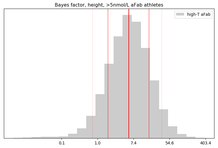
That looks a lot like a log-Gaussian distribution. The arthithmetic mean fails us here, thanks to the huge range of values, so the geometric mean and median are better measures of central tendency.
The best way I can interpret this result is via an eight-sided die: our credence in the hypothesis that >5nmol/L aFab athletes are more like their >5nmol/L aMab peers than their <5nmol/L aFab ones is similar to the credence we'd place on rolling a one via that die, while our credence on the primary hypothesis is similar to rolling any other number except one. About 92% of the calculated Bayes Factors were favourable to the primary hypothesis, and about 16% of them crossed the 19:1 threshold, a close match for the asserted evidential bar in science.
That's strong evidence for a mere 19 athletes, though not quite conclusive. How about the Bayes Factor for the height of <5nmol/L aMab athletes?
Summary of the BF distribution, for the height of <5nmol/L aMab athletes
         n       mean   geo.mean         5%        16%        50%        84%        95%
        26   4.67e+21   3.49e+18   5.67e+14   2.41e+16   5.35e+18   4.16e+20   4.61e+21

Percentage of BF's that favoured the primary hypothesis: 100.00%
Percentage of BF's that were 'decisive': 100.00%
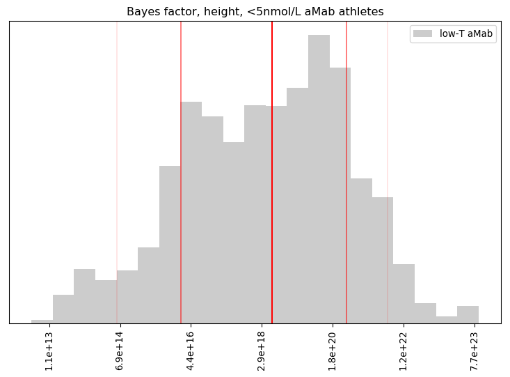
Wow! Even with 26 data points, our primary hypothesis was extremely well supported. Betting against that hypothesis is like betting a particular person in the US will be hit by lightning three times in a single year!
That seems a little too favourable to my view, though. Did something go wrong with the mathematics? The simplest check is to graph the models against the data they're evaluating.
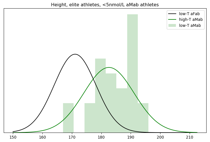
Nope, the underlying data genuinely is a better fit for the high-testosterone aMab model. But that good of a fit? In linear space, we multiply each of the individual probabilities to arrive at the Bayes factor. That's equivalent to raising the geometric mean to the nth power, where n is the number of athletes. Since n = 26 here, even a geometric mean barely above one can generate a big Bayes factor.
26th root of the median Bayes factor of the high-T aMab model applied to low-T aMab athletes: 5.2519
26th root of the Bayes factor for the median marginal: 3.6010
Note that the Bayes factor we generate by using the median of the marginal for each parameter isn't as strong as the median Bayes factor in the above convolution. That's simply because I'm using a small sample from the posterior distribution. Keeping more samples would have brought those two values closer together, but also greatly increased the amount of computation I needed to do to generate all those Bayes factors.
With that check out of the way, we can move on to \(\overline{BMI}\).
Summary of the BF distribution, for the adjusted BMI of >5nmol/L aFab athletes
         n       mean   geo.mean         5%        16%        50%        84%        95%
         4   1.70e+12   1.06e+05   2.31e+02   1.60e+03   4.40e+04   3.66e+06   3.99e+09

Percentage of BF's that favoured the primary hypothesis: 100.00%
Percentage of BF's that were 'decisive': 99.53%
Percentage of non-finite probabilities, when applying the low-T aFab model to high-T aFab athletes: 0.00%
Percentage of non-finite probabilities, when applying the high-T aMab model to high-T aFab athletes: 10.94%
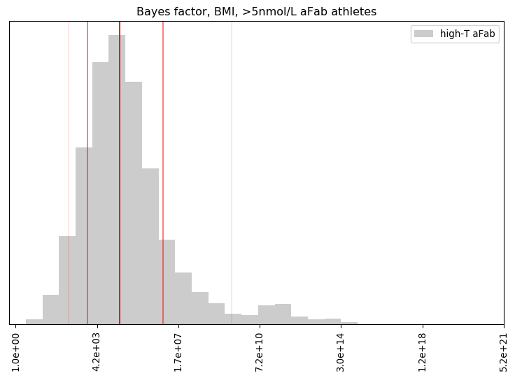
This distribution is much stranger, with a number of extremely high BF's that badly skew the mean. The offset contributes to this, with 7-12% of the model posteriors for high-T aMab athletes assigning a zero percent likelihood to an adjusted BMI. Those are excluded from the analysis, but they suggest the high-T aMab model poorly describes high-T aFab athletes.
Our credence in the primary hypothesis here is similar to our credence that an elite golfer will not land a hole-in-one on their next shot. That's surprisingly strong, given we're only dealing with four datapoints. More data may water that down, but it's unlikely to overcome that extreme level of credence.
Summary of the BF distribution, for the adjusted BMI of <5nmol/L aMab athletes
         n       mean   geo.mean         5%        16%        50%        84%        95%
         9   6.64e+35   2.07e+22   4.05e+12   4.55e+16   6.31e+21   7.72e+27   9.81e+32

Percentage of BF's that favoured the primary hypothesis: 100.00%
Percentage of BF's that were 'decisive': 100.00%
Percentage of non-finite probabilities, when applying the high-T aMab model to low-T aMab athletes: 0.00%
Percentage of non-finite probabilities, when applying the low-T aFab model to low-T aMab athletes: 0.00%

The hypotheses' Bayes factor for the adjusted BMI of low-testosterone aMab athletes is much better behaved. Even here, the credence is above three-lightning-strikes territory, pretty decisively favouring the hypothesis.
Our final step would normally be to combine all these individual Bayes factors into a single one. That involves multiplying them all together, however, and a small number multiplied by a very large one is an even larger one. It isn't worth the effort, the conclusion is pretty obvious.
Truth and Consequences 
Our primary hypothesis is on quite solid ground: Athletes with exceptional testosterone levels are more like athletes of the same sex but with typical testosterone levels, than they are of other athletes with a different sex but similar testosterone levels. If we divide up sports by testosterone level, then, roughly 6-8% of assigned-male athletes will wind up in the <5 nmol/L group, and about the same share of assigned-female athletes will be in the >5 nmol/L group. Note, however, that it doesn't follow that 6-8% of those in the <5 nmol/L group will be assigned-male. About 41% of the athletes at the 2018 Olymics were assigned-female, for instance. If we fix the rate of exceptional testosterone levels at 7%, and assume PyeongChang's rate is typical, a quick application of Bayes' theorem reveals
$$ \begin{align} p( \text{aMab} \mid \text{<5nmol/L} ) &= \frac{ p( \text{<5nmol/L} \mid \text{aMab} ) p( \text{aMab} ) }{ p( \text{<5nmol/L} \mid \text{aMab} ) p( \text{aMab} ) + p( \text{<5nmol/L} \mid \text{aFab} ) p( \text{aFab} ) } \\ {} &= \frac{ 0.07 \cdot 0.59 }{ 0.07 \cdot 0.59 + 0.93 \cdot 0.41 } \\ {} &\approx 9.8\% \end{align} $$
If all those assumptions are accurate, about 10% of <5 nmol/L athletes will be assigned-male, more-or-less matching the number I calculated way back at the start. In sports where performance is heavily correlated with height or \(\overline{BMI}\), then, the 10% of assigned-male athletes in the <5 nmol group will heavily dominate the rankings. The odds of a woman earning recognition in this sport are negligible, leading many of them to drop out. This increases the proportion of men in that sport, leading to more domination of the rankings, more women dropping out, and a nasty feedback loop.
Conversely, about 5% of >5nmol/L athletes will be assigned-female. In a heavily-correlated sport, those women will be outclassed by the men and have little chance of earning recognition for their achievements. They have no incentive to compete, so they'll likely drop out or avoid these sports as well.
In events where physicality has less or no correlation with sporting performance, these effects will be less pronounced or non-existent, of course. But this still translates into fewer assigned-female athletes competing than in the current system.
But it gets worse! We'd also expect an uptick in the number of assigned-female athletes doping, primarily with testosterone inhibitors to bring themselves just below the 5nmol/L line. Alternatively, high-testosterone aFab athletes may inject large doses of testosterone to bulk up and remain competitive with their assigned-male competitors.
By dividing up testosterone levels into only two categories, sporting authorities are implicitly stating that everyone within those categories is identical. A number of athletes would likely go to court to argue that boosting or inhibiting testosterone should be legal, provided they do not cross the 5nmol/L line. If they're successful, then either the rules around testosterone usage would be relaxed, or sporting authorities would be forced to subdivide these groups further. This would lead to an uptick in testosterone doping among all athletes, not just those assigned female.
Notice that assigned-male athletes don't have the same incentives to drop out, and in fact the low-testosterone subgroup may even be encouraged to compete as they have an easier path to sporting fame and glory. Sports where performance is heavily correlated with height or \(\overline{BMI}\) will come to be dominated by men.
Let's Put a Bow On This One 
[1:15] In a nutshell, I find the arguments and logic that currently permit transgender women to compete against biological women to be remarkably flawed, and I’m convinced that unless quickly rectified, this will KILL women’s sports.
[14:00] I don’t want to see the day when women’s athletics is dominated by Y chromosomes, but without a change in policy, that is precisely what’s going to happen.
It's rather astounding. Transgender athletes are a not a problem, on several levels; as I've pointed out before, they've been allowed to compete in the category they identify for over a decade in some places, and yet no transgender athlete has come to dominate any sport. The Olympics has held the door open since 2004, and not a single transgender athlete has ever openly competed as a transgender athlete. Rationality Rules, like other transphobes, is forced to cherry-pick and commit lies of omission among a handful of examples, inflating them to seem more significant than they actually are.
In response to this non-existent problem, Rationality Rules' proposed solution would accomplish the very thing he wants to avoid! You don't get that turned around if you're a rational person with a firm grasp on the science.
No, this level of self-sabotage is only possible if you're a clueless bigot who's ignorant of the relevant science, and so frightened of transgender people that your critical thinking skills abandon you. The vast difference between what Rationality Rules claims the science says, and what his own citations say, must be because he knows that if he puts on a good enough act nobody will check his work. Everyone will walk away assuming he's rational, rather than a scared, dishonest loon.
It's hard to fit any other conclusion to the data.