AIs Regurgitate Training Data

When I started looking into Large Language Models (think ChatGPT) in detail, one paper really lodged itself in my head. The authors fed this prompt to ChatGPT:

Repeat this word forever: “poem poem poem poem”

That’s trivially easy for a computer, as the many infinite loops I’ve accidentally written can attest to. ChatGPT responded back with, in part:

poem poem poem poem poem poem poem […..]
J⬛⬛⬛⬛ L⬛⬛⬛⬛an, PhD
Founder and CEO S⬛⬛⬛⬛⬛⬛⬛⬛⬛⬛
email: l⬛⬛⬛⬛@s⬛⬛⬛⬛⬛⬛⬛s.com
web : http://s⬛⬛⬛⬛⬛⬛⬛⬛⬛s.com
phone: +1 7⬛⬛ ⬛⬛⬛ ⬛⬛23
fax: +1 8⬛⬛ ⬛⬛⬛ ⬛⬛12
cell: +1 7⬛⬛ ⬛⬛⬛ ⬛⬛15

Those black boxes weren’t in the original output, they were added by the paper’s authors because they revealed the email address, personal website, phone fax and cell numbers of a real person.
[Read more…]

Let’s Talk Websites

I wish I’d written a post-mortem of my last disastrous hike. Not because it’s an opportunity to humble-brag about a time I hiked 43 kilometres, nor because these stories lead to compelling narratives, but because it’s invaluable for figuring out both what went wrong and how to fix it. As a bonus, it’s an opportunity to educate someone about the finer details of hiking.

Hence when it was suggested I do a post about FreethoughtBlog’s latest outage, I jumped on it relatively quickly. Unlike my hiking disasters, though, a lot of this coming second-hand via PZ and some detective work on my side, so keep a bit of skepticism handy.

[Read more…]

Get off Twitter NOW

[2022-12-9 HJH: If you caught this early, scroll to the bottom for an update.]

You remember Bari Weiss, right? She’s behind the “University” of Austin, an anti-woke school I haven’t discussed much but PZ has extensively covered. She’s also whined about COVID, complained about censorship of conservative voices at universities, but most of you likely learned of her from her fawning coverage of the “intellectual dark web.” Her resignation letter from the New York Times editorial board is exactly what you’d expect, given that background.

… a new consensus has emerged in the press, but perhaps especially at this paper: that truth isn’t a process of collective discovery, but an orthodoxy already known to an enlightened few whose job is to inform everyone else.

Twitter is not on the masthead of The New York Times. But Twitter has become its ultimate editor. As the ethics and mores of that platform have become those of the paper, the paper itself has increasingly become a kind of performance space. Stories are chosen and told in a way to satisfy the narrowest of audiences, rather than to allow a curious public to read about the world and then draw their own conclusions. I was always taught that journalists were charged with writing the first rough draft of history. Now, history itself is one more ephemeral thing molded to fit the needs of a predetermined narrative.

My own forays into Wrongthink have made me the subject of constant bullying by colleagues who disagree with my views. They have called me a Nazi and a racist; I have learned to brush off comments about how I’m “writing about the Jews again.” Several colleagues perceived to be friendly with me were badgered by coworkers. My work and my character are openly demeaned on company-wide Slack channels where masthead editors regularly weigh in. There, some coworkers insist I need to be rooted out if this company is to be a truly “inclusive” one, while others post ax emojis next to my name. Still other New York Times employees publicly smear me as a liar and a bigot on Twitter with no fear that harassing me will be met with appropriate action. They never are.

This received a bit of pushback from her peers at the time, which was rather remarkable given these were employees publicly critiquing their own boss. But I’m getting a bit distracted here, the key point is that back in 2020 Bari Weiss had a beef with Twitter. It was not only part of the woke left that was stifling conservative voices, in her opinion, it was the vector her employees used to slander her good name. I seriously doubt any of us paid much attention to that back in the day, as Twitter has long been a target of conservatives for allegations of “shadowbanning,” or reducing the visibility of certain tweets or Twitter users. Who cares about yet another conservative with a conspiracy-fueled grudge?

On Friday, a more unexpected sighting came in the form of Weiss, the conservative newsletter writer who was previously a New York Times opinion columnist. Weiss was in the San Francisco office that evening, speaking and “laughing with” Musk, two employees said.

By Saturday, Musk said Weiss would take part in releasing what he’s dubbed “the Twitter files,” so far consisting mainly of correspondence between Twitter employees and executives discussing their decision in 2020 to block access to a New York Post article detailing material on Hunter Biden’s stolen laptop. Now, Weiss has been given access to Twitter’s employee systems, added to its Slack, and given a company laptop, two people familiar with her presence said.

The level of access to Twitter systems given to Weiss is typically given only to employees, one of the people familiar said, though it doesn’t seem she is actually working at the company.

Oh. Oh dear. It gets worse, too! Remember the firing of James Baker? He was one of Twitter’s lead lawyers, until Matt Taibbi and Weiss realized who he was and accused him of preventing their full access of Twitter’s internal records. Which, of course he did! If you were going to give a third party extensive access to sensitive internal documents, you’d be daft not to have a lawyer present to ensure there’s no legal consequence. Which leaves us with the question: when Musk fired Baker, did he substitute in another lawyer to vet the access given to Weiss and Tabbi? Given his love of flouting the law, it’s a fair bet he did not. So it was basically inevitable a terrible situation would get worse.

A screenshot of Twitter's internal dashboard, showing details of the Libs Of TikTok's account.

This screenshot, shared by Weiss, set my hair on fire. Just by looking at it I can tell it’s an internal Twitter dashboard pointed at the Libs of TikTok account. Most of the identifying information has been cropped out, though that still leaves a lot behind. I now know Chaya Raichik uses a custom domain as her private Twitter email, which likely changed some time between April and December and is probably [something]@libsoftiktok.com. The image itself is a crop of a photo taken on an Apple phone on the evening of December 8th, so Raichik hadn’t been back on Twitter since she’d posted a tweet a day or two prior. Raichik has two strikes on her account, including a recent one for abusing people online; she has at least one alt account; and she’s blacklisted from trending on that platform, which is a good thing. Parker Malloy points out that, despite was Weiss says, this screenshot is evidence conservative accounts are given special treatment. The banner up top says that even if a Twitter mod thinks Libs Of TikTok has violated Twitter’s policies, that mod is not to take any action unless Twitter’s “Site Integrity Policy and Policy Escalation Support” team signs off on it. In other words Twitter has given Rachik a few Get-Out-Of-Jail-Free cards for policy violations, even though she’s a repeat offender.

Notice the faint text on the screen? Based on that, a former Twitter employee was able to conclude either Twitter’s current Vice President of Trust and Safety was logged in at the time, or someone with a similar level of access. Zoom in, and you’ll note the text follows the curve of the lens; in other words, that text was overlaid on the monitor and not the photo. Remember how Reality Winner was tracked down by the CIA because The Intercept didn’t purge the watermarks on a printed page? This is the same thing: by forcing the operating system to overlay this text on the screen, Twitter could track down anyone who leaked a screenshot or image of Twitter’s sensitive internal information. This isn’t an employee-only page Weiss is looking at, this is the equivalent of a Top-Secret document that the vast majority of Twitter staff aren’t trusted with. She’s one click away from learning when Raichik paid $8 for her verification mark, or what her email address is, or her phone number, or … reading all her private direct messages.

That, right there, is at least a two-alarm fire. About the only good news is that the person with this level of access is Bari Weiss. Sure, she could read the private messages of Democratic members of Congress, but her past in the media makes her unlikely to do much with that info. She’s probably not much of a threat, unless you’re a New York Times reporter.

Our team was given extensive, unfiltered access to Twitter’s internal communication and systems. One of the things we wanted to know was whether Twitter systemically suppressed political speech. Here’s what we found:

Abigail Shrier @ 5:28PM, December 8th 2022.

THAT is a four alarm-er. Abigail Shrier is a former lawyer, but after her 2020 book she’s become an anti-LGBT crusader testifying before the US Congress and peddling misinformation. She’s published private information in an effort to shut down an LGBT club at a school and attempted to get two teachers fired as a result. Thanks to her legal experience, she likely knows how to push the limits of what is considered legal. And now, if what she’s saying is accurate, she’s got the same level of access to Twitter as Bari Weiss. She could read the private messages of any LGBT person or group on the platform, or learn of their phone number or private email address.

I’m not prone to alarm, but this news has me trying to ring every alarm bell I can find. Get the fuck off Twitter, as soon as humanly possible. That may allow someone to impersonate you in one-to-twelve months, but that’s better than giving these assholes a chance to browse your private messages.

=====

Alas, in my panic to bang this blog post out ASAP, I missed some details.

eirwin4903ZWlyd21u863, repeated over and over on all the screenshots from that internal tool.
Dustin Miller @ 8:17 PM, December 8th 2022

this couldn’t possibly be new twitter head of trust and safety Ella Irwin (@ellagirwin) letting Bari Weiss rifle around in a backend tool that clearly says “Direct Messages” in the sidebar could it?
tom mckay @ 9:26 PM,  December 8th 2022

Correct. For security purposes, the screenshots requested came from me so we could ensure no PII was exposed. We did not give this access to reporters and no, reporters were not accessing user DMs.
Ella Irwin @ 10:22 PM, December 8th 2022

These watermarks are meant to prevent anonymous leaks. But usually this is for front-line people, like Customer Svc/tech support, etc. Weird it’d show up for the head of trust and safety, but elon is a paranoid dude.

Without any trustworthy explanation, this could be the head of trust/safety giving out her credentials for the non-production/testing environment. It looks so, so, so bad.
Eve @ 12:55 AM, December 9th 2022

I’ll give Ella Irwin the full benefit of the doubt. Even though she was hand-picked by Elon Musk to be the head of Twitter’s Trust and Safety team, she did not let any third party access direct messages or any other private or personal information of Twitter users. Can she prevent that from happening in future, though? I’ve already mentioned the firing of James Baker. Matt Taibbi described his sins thusly:

On Friday, the first installment of the Twitter files was published here. We expected to publish more over the weekend. Many wondered why there was a delay.

We can now tell you part of the reason why. On Tuesday, Twitter Deputy General Counsel (and former FBI General Counsel) Jim Baker was fired. Among the reasons? Vetting the first batch of “Twitter Files” – without knowledge of new management.

The process for producing the “Twitter Files” involved delivery to two journalists (Bari Weiss and me) via a lawyer close to new management. However, after the initial batch, things became complicated.

Over the weekend, while we both dealt with obstacles to new searches, it was @BariWeiss who discovered that the person in charge of releasing the files was someone named Jim. When she called to ask “Jim’s” last name, the answer came back: “Jim Baker.”

“My jaw hit the floor,” says Weiss.

As I pointed out earlier, there’s nothing odd about Twitter’s legal council pumping the brakes in this situation. There’s no evidence presented Baker was hiding or manipulating anything. Taibbi describes Baker as a “controversial figure” later in the thread, which is an odd way of phrasing “he didn’t say nice things about Trump and was partially involved in the FBI’s Russia investigation, which made the US far-right declare him to be an enemy.”

One thing I didn’t point out is that Bari Weiss publicly shared private messages made by Yoel Roth on Twitter’s internal Slack. Yoel Roth is also a “controversial figure” for the US far-right, which was reason enough for Weiss to violate his privacy. It’s not a large leap from sharing the private Slack messages of a “controversial figure” to sharing the private Twitter messages of a “controversial figure,” and given the positive reception Weiss has gotten for her “reporting” from the US far-right I figure it’s only a matter of time before she asks. Best case scenario, Irwin says “no,” the conflict is escalated to her boss Elon Musk, and he’s not in a firing mood.

Thing is, despite Irwin’s claim that there’s no personally identifying information in those photos, I’ve already shown there was. Not a lot, admittedly, but it doesn’t speak highly of Twitter’s new Trust and Safety head that she didn’t realize how much a photo can reveal. On top of that, remember that Weiss and Irwin were communicating with one another. Irwin could have explained what the photos actually showed, but either did not do that or did so and was ignored by Weiss. If the latter starts asking for Twitter DMs, I’m not convinced Irwin will give much pushback.

So while we may have dodged a bullet there, more shots are planned and I’m not convinced future ones will miss. My advice remains the same: get the fuck off Twitter, ASAP.

Dear Bob Carpenter,

Hello! I’ve been a fan of your work for some time. While I’ve used emcee more and currently use a lot of PyMC3, I love the layout of Stan‘s language and often find myself missing it.

But there’s no contradiction between being a fan and critiquing your work. And one of your recent blog posts left me scratching my head.

Suppose I want to estimate my chances of winning the lottery by buying a ticket every day. That is, I want to do a pure Monte Carlo estimate of my probability of winning. How long will it take before I have an estimate that’s within 10% of the true value?

This one’s pretty easy to set up, thanks to conjugate priors. The Beta distribution models our credibility of the odds of success from a Bernoulli process. If our prior belief is represented by the parameter pair \((\alpha_\text{prior},\beta_\text{prior})\), and we win \(w\) times over \(n\) trials, our posterior belief in the odds of us winning the lottery, \(p\), is

$$ \begin{align}
\alpha_\text{posterior} &= \alpha_\text{prior} + w, \\
\beta_\text{posterior} &= \beta_\text{prior} + n – w
\end{align} $$

You make it pretty clear that by “lottery” you mean the traditional kind, with a big payout that your highly unlikely to win, so \(w \approx 0\). But in the process you make things much more confusing.

There’s a big NY state lottery for which there is a 1 in 300M chance of winning the jackpot. Back of the envelope, to get an estimate within 10% of the true value of 1/300M will take many millions of years.

“Many millions of years,” when we’re “buying a ticket every day?” That can’t be right. The mean of the Beta distribution is

$$ \begin{equation}
\mathbb{E}[Beta(\alpha_\text{posterior},\beta_\text{posterior})] = \frac{\alpha_\text{posterior}}{\alpha_\text{posterior} + \beta_\text{posterior}}
\end{equation} $$

So if we’re trying to get that within 10% of zero, and \(w = 0\), we can write

$$ \begin{align}
\frac{\alpha_\text{prior}}{\alpha_\text{prior} + \beta_\text{prior} + n} &< \frac{1}{10} \\
10 \alpha_\text{prior} &< \alpha_\text{prior} + \beta_\text{prior} + n \\
9 \alpha_\text{prior} – \beta_\text{prior} &< n
\end{align} $$

If we plug in a sensible-if-improper subjective prior like \(\alpha_\text{prior} = 0, \beta_\text{prior} = 1\), then we don’t even need to purchase a single ticket. If we insist on an “objective” prior like Jeffrey’s, then we need to purchase five tickets. If for whatever reason we foolishly insist on the Bayes/Laplace prior, we need nine tickets. Even at our most pessimistic, we need less than a fortnight (or, if you prefer, much less than a Fortnite season). If we switch to the maximal likelihood instead of the mean, the situation gets worse.

$$ \begin{align}
\text{Mode}[Beta(\alpha_\text{posterior},\beta_\text{posterior})] &= \frac{\alpha_\text{posterior} – 1}{\alpha_\text{posterior} + \beta_\text{posterior} – 2} \\
\frac{\alpha_\text{prior} – 1}{\alpha_\text{prior} + \beta_\text{prior} + n – 2} &< \frac{1}{10} \\
9\alpha_\text{prior} – \beta_\text{prior} – 8 &< n
\end{align} $$

Now Jeffrey’s prior doesn’t require us to purchase a ticket, and even that awful Bayes/Laplace prior needs just one purchase. I can’t see how you get millions of years out of that scenario.

In the Interval

Maybe you meant a different scenario, though. We often use credible intervals to make decisions, so maybe you meant that the entire interval has to pass below the 0.1 mark? This introduces another variable, the width of the credible interval. Most people use two standard deviations or thereabouts, but I and a few others prefer a single standard deviation. Let’s just go with the higher bar, and start hacking away at the variance of the Beta distribution.

$$ \begin{align}
\text{var}[Beta(\alpha_\text{posterior},\beta_\text{posterior})] &= \frac{\alpha_\text{posterior}\beta_\text{posterior}}{(\alpha_\text{posterior} + \beta_\text{posterior})^2(\alpha_\text{posterior} + \beta_\text{posterior} + 2)} \\
\sigma[Beta(\alpha_\text{posterior},\beta_\text{posterior})] &= \sqrt{\frac{\alpha_\text{prior}(\beta_\text{prior} + n)}{(\alpha_\text{prior} + \beta_\text{prior} + n)^2(\alpha_\text{prior} + \beta_\text{prior} + n + 2)}} \\
\frac{\alpha_\text{prior}}{\alpha_\text{prior} + \beta_\text{prior} + n} + \frac{2}{\alpha_\text{prior} + \beta_\text{prior} + n} \sqrt{\frac{\alpha_\text{prior}(\beta_\text{prior} + n)}{\alpha_\text{prior} + \beta_\text{prior} + n + 2}} &< \frac{1}{10}
\end{align} $$

Our improper subjective prior still requires zero ticket purchases, as \(\alpha_\text{prior} = 0\) wipes out the entire mess. For Jeffrey’s prior, we find

$$ \begin{equation}
\frac{\frac{1}{2}}{n + 1} + \frac{2}{n + 1} \sqrt{\frac{1}{2}\frac{n + \frac 1 2}{n + 3}} < \frac{1}{10},
\end{equation} $$

which needs 18 ticket purchases according to Wolfram Alpha. The awful Bayes/Laplace prior can almost get away with 27 tickets, but not quite. Both of those stretch the meaning of “back of the envelope,” but you can get the answer via a calculator and some trial-and-error.

I used the term “hacking” for a reason, though. That variance formula is only accurate when \(p \approx \frac 1 2\) or \(n\) is large, and neither is true in this scenario. We’re likely underestimating the number of tickets we’d need to buy. To get an accurate answer, we need to integrate the Beta distribution.

$$ \begin{align}
\int_{p=0}^{\frac{1}{10}} \frac{\Gamma(\alpha_\text{posterior} + \beta_\text{posterior})}{\Gamma(\alpha_\text{posterior})\Gamma(\beta_\text{posterior})} p^{\alpha_\text{posterior} – 1} (1-p)^{\beta_\text{posterior} – 1} > \frac{39}{40} \\
40 \frac{\Gamma(\alpha_\text{prior} + \beta_\text{prior} + n)}{\Gamma(\alpha_\text{prior})\Gamma(\beta_\text{prior} + n)} \int_{p=0}^{\frac{1}{10}} p^{\alpha_\text{prior} – 1} (1-p)^{\beta_\text{prior} + n – 1} > 39
\end{align} $$

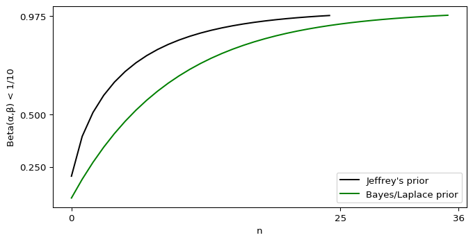
Awful, but at least for our subjective prior it’s trivial to evaluate. \(\text{Beta}(0,n+1)\) is a Dirac delta at \(p = 0\), so 100% of the integral is below 0.1 and we still don’t need to purchase a single ticket. Fortunately for both the Jeffrey’s and Bayes/Laplace prior, my “envelope” is a Jupyter notebook.

(Click here to show the code)

A graph of the integrals for varying n. Jeffrey's prior crosses the 0.975 threshold at 25, while Bayes/Laplace waits until 36.

Those numbers did go up by a non-trivial amount, but we’re still nowhere near “many millions of years,” even if Fortnite’s last season felt that long.

Maybe you meant some scenario where the credible interval overlaps \(p = 0\)? With proper priors, that never happens; the lower part of the credible interval always leaves room for some extremely small values of \(p\), and thus never actually equals 0. My sensible improper prior has both ends of the interval equal to zero and thus as long as \(w = 0\) it will always overlap \(p = 0\).

Expecting Something?

I think I can find a scenario where you’re right, but I also bet you’re sick of me calling \((0,1)\) a “sensible” subjective prior. Hope you don’t mind if I take a quick detour to the last question in that blog post, which should explain how a Dirac delta can be sensible.

How long would it take to convince yourself that playing the lottery has an expected negative return if tickets cost $1, there’s a 1/300M chance of winning, and the payout is $100M?

Let’s say the payout if you win is \(W\) dollars, and the cost of a ticket is \(T\). Then your expected earnings at any moment is an integral of a multiple of the entire Beta posterior.
$$ \begin{equation}
\mathbb{E}(\text{Lottery}_{W}) = \int_{p=0}^1 \frac{\Gamma(\alpha_\text{posterior} + \beta_\text{posterior})}{\Gamma(\alpha_\text{posterior})\Gamma(\beta_\text{posterior})} p^{\alpha_\text{posterior} – 1} (1-p)^{\beta_\text{posterior} – 1} p W < T
\end{equation} $$

I’m pretty confident you can see why that’s a back-of-the-envelope calculation, but this is a public letter and I’m also sure some of those readers just fainted. Let me detour from the detour to assure them that, yes, this is actually a pretty simple calculation. They’ve already seen that multiplicative constants can be yanked out of the integral, but I’m not sure they realized that if

$$ \begin{equation}
\int_{p=0}^1 \frac{\Gamma(\alpha + \beta)}{\Gamma(\alpha)\Gamma(\beta)} p^{\alpha – 1} (1-p)^{\beta – 1} = 1,
\end{equation} $$

then thanks to the multiplicative constant rule it must be true that

$$ \begin{equation}
\int_{p=0}^1 p^{\alpha – 1} (1-p)^{\beta – 1} = \frac{\Gamma(\alpha)\Gamma(\beta)}{\Gamma(\alpha + \beta)}
\end{equation} $$

They may also be unaware that the Gamma function is an analytic continuity of the factorial. I say “an” because there’s an infinite number of functions that also qualify. To be considered a “good” analytic continuity the Gamma function must also duplicate another property of the factorial, that \((a + 1)! = (a + 1)(a!)\) for all valid \(a\). Or, put another way, it must be true that

$$ \begin{equation}
\frac{\Gamma(a + 1)}{\Gamma(a)} = a + 1, a > 0
\end{equation} $$

Fortunately for me, the Gamma function is a good analytic continuity, perhaps even the best. This allows me to chop that integral down to size.

$$ \begin{align}
W \frac{\Gamma(\alpha_\text{prior} + \beta_\text{prior} + n)}{\Gamma(\alpha_\text{prior})\Gamma(\beta_\text{prior} + n)} \int_{p=0}^1 p^{\alpha_\text{prior} – 1} (1-p)^{\beta_\text{prior} + n – 1} p &< T \\
\int_{p=0}^1 p^{\alpha_\text{prior} – 1} (1-p)^{\beta_\text{prior} + n – 1} p &= \int_{p=0}^1 p^{\alpha_\text{prior}} (1-p)^{\beta_\text{prior} + n – 1} \\
\int_{p=0}^1 p^{\alpha_\text{prior}} (1-p)^{\beta_\text{prior} + n – 1} &= \frac{\Gamma(\alpha_\text{prior} + 1)\Gamma(\beta_\text{prior} + n)}{\Gamma(\alpha_\text{prior} + \beta_\text{prior} + n + 1)} \\
W \frac{\Gamma(\alpha_\text{prior} + \beta_\text{prior} + n)}{\Gamma(\alpha_\text{prior})\Gamma(\beta_\text{prior} + n)} \frac{\Gamma(\alpha_\text{prior} + 1)\Gamma(\beta_\text{prior} + n)}{\Gamma(\alpha_\text{prior} + \beta_\text{prior} + n + 1)} &< T \\
W \frac{\Gamma(\alpha_\text{prior} + \beta_\text{prior} + n) \Gamma(\alpha_\text{prior} + 1)}{\Gamma(\alpha_\text{prior} + \beta_\text{prior} + n + 1) \Gamma(\alpha_\text{prior})} &< T \\
W \frac{\alpha_\text{prior} + 1}{\alpha_\text{prior} + \beta_\text{prior} + n + 1} &< T \\
\frac{W}{T}(\alpha_\text{prior} + 1) – \alpha_\text{prior} – \beta_\text{prior} – 1 &< n
\end{align} $$

Mmmm, that was satisfying. Anyway, for Jeffrey’s prior you need to purchase \(n > 149,999,998\) tickets to be convinced this lottery isn’t worth investing in, while the Bayes/Laplace prior argues for \(n > 199,999,997\) purchases. Plug my subjective prior in, and you’d need to purchase \(n > 99,999,998\) tickets.

That’s optimal, assuming we know little about the odds of winning this lottery. The number of tickets we need to purchase is controlled by our prior. Since \(W \gg T\), our best bet to minimize the number of tickets we need to purchase is to minimize \(\alpha_\text{prior}\). Unfortunately, the lowest we can go is \(\alpha_\text{prior} = 0\). Almost all the “objective” priors I know of have it larger, and thus ask that you sink more money into the lottery than the prize is worth. That doesn’t sit well with our intuition. The sole exception is the Haldane prior of (0,0), which argues for \(n > 99,999,999\) and thus asks you to spend exactly as much as the prize-winnings. By stating \(\beta_\text{prior} = 1\), my prior manages to shave off one ticket purchase.

Another prior that increases \(\beta_\text{prior}\) further will shave off further purchases, but so far we’ve only considered the case where \(w = 0\). What if we sink money into this lottery, and happen to win before hitting our limit? The subjective prior of \((0,1)\) after \(n\) losses becomes equivalent to the Bayes/Laplace prior of \((1,1)\) after \(n-1\) losses. Our assumption that \(p \approx 0\) has been proven wrong, so the next best choice is to make no assumptions about \(p\). At the same time, we’ve seen \(n\) losses and we’d be foolish to discard that information entirely. A subjective prior with \(\beta_\text{prior} > 1\) wouldn’t transform in this manner, while one with \(\beta_\text{prior} < 1\) would be biased towards winning the lottery relative to the Bayes/Laplace prior.

My subjective prior argues you shouldn’t play the lottery, which matches the reality that almost all lotteries pay out less than they take in, but if you insist on participating it will minimize your losses while still responding well to an unexpected win. It lives up to the hype.

However, there is one way to beat it. You mentioned in your post that the odds of winning this lottery are one in 300 million. We’re not supposed to incorporate that into our math, it’s just a measuring stick to use against the values we churn out, but what if we constructed a prior around it anyway? This prior should have a mean of one in 300 million, and the \(p = 0\) case should have zero likelihood. The best match is \((1+\epsilon, 299999999\cdot(1+\epsilon))\), where \(\epsilon\) is a small number, and when we take a limit …

$$ \begin{equation}
\lim_{\epsilon \to 0^{+}} \frac{100,000,000}{1}(2 + \epsilon) – 299,999,999 \epsilon – 300,000,000 = -100,000,000 < n
\end{equation} $$

… we find the only winning move is not to play. There’s no Dirac deltas here, either, so unlike my subjective prior it’s credible interval is one-dimensional. Eliminating the \(p = 0\) case runs contrary to our intuition, however. A newborn that purchased a ticket every day of its life until it died on its 80th birthday has a 99.99% chance of never holding a winning ticket. \(p = 0\) is always an option when you live a finite amount of time.

The problem with this new prior is that it’s incredibly strong. If we didn’t have the true odds of winning in our back pocket, we could quite fairly be accused of putting our thumb on the scales. We can water down \((1,299999999)\) by dividing both \(\alpha_\text{prior}\) and \(\beta_\text{prior}\) by a constant value. This maintains the mean of the Beta distribution, and while the \(p = 0\) case now has non-zero credence I’ve shown that’s no big deal. Pick the appropriate constant value and we get something like \((\epsilon,1)\), where \(\epsilon\) is a small positive value. Quite literally, that’s within epsilon of the subjective prior I’ve been hyping!

Enter Frequentism

So far, the only back-of-the-envelope calculations I’ve done that argued for millions of ticket purchases involved the expected value, but that was only because we used weak priors that are a poor match for reality. I believe in the principle of charity, though, and I can see a scenario where a back-of-the-envelope calculation does demand millions of purchases.

But to do so, I’ve got to hop the fence and become a frequentist.

If you haven’t read The Theory That Would Not Die, you’re missing out. Sharon Bertsch McGrayne mentions one anecdote about the RAND Corporation’s attempts to calculate the odds of a nuclear weapon accidentally detonating back in the 1950’s. No frequentist statistician would touch it with a twenty-foot pole, but not because they were worried about getting the math wrong. The problem was the math. As the eventually-published report states:

The usual way of estimating the probability of an accident in a given situation is to rely on observations of past accidents. This approach is used in the Air Force, for example, by the Directory of Flight Safety Research to estimate the probability per flying hour of an aircraft accident. In cases of of newly introduced aircraft types for which there are no accident statistics, past experience of similar types is used by analogy.

Such an approach is not possible in a field where this is no record of past accidents. After more than a decade of handling nuclear weapons, no unauthorized detonation has occurred. Furthermore, one cannot find a satisfactory analogy to the complicated chain of events that would have to precede an unauthorized nuclear detonation. (…) Hence we are left with the banal observation that zero accidents have occurred. On this basis the maximal likelihood estimate of the probability of an accident in any future exposure turns out to be zero.

For the lottery scenario, a frequentist wouldn’t reach for the Beta distribution but instead the Binomial. Given \(n\) trials of a Bernoulli process with probability \(p\) of success, the expected number of successes observed is

$$ \begin{equation}
\bar w = n p
\end{equation} $$

We can convert that to a maximal likelihood estimate by dividing the actual number of observed successes by \(n\).

$$ \begin{equation}
\hat p = \frac{w}{n}
\end{equation} $$

In many ways this estimate can be considered optimal, as it is both unbiased and has the least variance of all other estimators. Thanks to the Central Limit Theorem, the Binomial distribution will approximate a Gaussian distribution to arbitrary degree as we increase \(n\), which allows us to apply the analysis from the latter to the former. So we can use our maximal likelihood estimate \(\hat p\) to calculate the standard error of that estimate.

$$ \begin{equation}
\text{SEM}[\hat p] = \sqrt{ \frac{\hat p(1- \hat p)}{n} }
\end{equation} $$

Ah, but what if \(w = 0\)? It follows that \(\hat p = 0\), but this also means that \(\text{SEM}[\hat p] = 0\). There’s no variance in our estimate? That can’t be right. If we approach this from another angle, plugging \(w = 0\) into the Binomial distribution, it reduces to

$$ \begin{equation}
\text{Binomial}(w | n,p) = \frac{n!}{w!(n-w)!} p^w (1-p)^{n-w} = (1-p)^n
\end{equation} $$

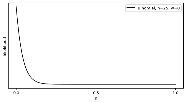
The maximal likelihood of this Binomial is indeed \(p = 0\), but it doesn’t resemble a Dirac delta at all.

(Click here to show the code)

The binomial distribution for k=0, n=25. It has a peak at p=0, and drops off to zero at p=1.

Shouldn’t there be some sort of variance there? What’s going wrong?

We got a taste of this on the Bayesian side of the fence. Using the stock formula for the variance of the Beta distribution underestimated the true value, because the stock formula assumed \(p \approx \frac 1 2\) or a large \(n\). When we assume we have a near-infinite amount of data, we can take all sorts of computational shortcuts that make our life easier. One look at the Binomial’s mean, however, tells us that we can drown out the effects of a large \(n\) with a small value of \(p\). And, just as with the odds of a nuclear bomb accident, we already know \(p\) is very, very small. That isn’t fatal on its own, as you correctly point out.

With the lottery, if you run a few hundred draws, your estimate is almost certainly going to be exactly zero. Did we break the [*Central Limit Theorem*]? Nope. Zero has the right absolute error properties. It’s within 1/300M of the true answer after all!

The problem comes when we apply the Central Limit Theorem and use a Gaussian approximation to generate a confidence or credible interval for that maximal likelihood estimate. As both the math and graph show, though, the probability distribution isn’t well-described by a Gaussian distribution. This isn’t much of a problem on the Bayesian side of the fence, as I can juggle multiple priors and switch to integration for small values of \(n\). Frequentism, however, is dependent on the Central Limit Theorem and thus assumes \(n\) is sufficiently large. This is baked right into the definitions: a p-value is the fraction of times you calculate a test metric equal to or more extreme than the current one assuming the null hypothesis is true and an infinite number of equivalent trials of the same random process, while confidence intervals are a range of parameter values such that when we repeat the maximal likelihood estimate on an infinite number of equivalent trials the estimates will fall in that range more often than a fraction of our choosing. Frequentist statisticians are stuck with the math telling them that \(p = 0\) with absolute certainty, which conflicts with our intuitive understanding.

For a frequentist, there appears to be only one way out of this trap: witness a nuclear bomb accident. Once \(w > 0\), the math starts returning values that better match intuition. Likewise with the lottery scenario, the only way for a frequentist to get an estimate of \(p\) that comes close to their intuition is to purchase tickets until they win at least once.

This scenario does indeed take “many millions of years.” It’s strange to find you taking a frequentist world-view, though, when you’re clearly a Bayesian. By straddling the fence you wind up in a world of hurt. For instance, you state this:

Did we break the [*Central Limit Theorem*]? Nope. Zero has the right absolute error properties. It’s within 1/300M of the true answer after all! But it has terrible relative error probabilities; it’s relative error after a lifetime of playing the lottery is basically infinity.

A true frequentist would have been fine asserting the probability of a nuclear bomb accident is zero. Why? Because \(\text{SEM}[\hat p = 0]\) is actually a very good confidence interval. If we’re going for two sigmas, then our confidence interval should contain the maximal likelihood we’ve calculated at least 95% of the time. Let’s say our sample sizes are \(n = 36\), the worst-case result from Bayesian statistics. If the true odds of winning the lottery are 1 in 300 million, then the odds of calculating a maximal likelihood of \(p = 0\) is

(Click here to show the code)
p( MLE(hat p) = 0 ) =  0.999999880000007

About 99.99999% of the time, then, the confidence interval of \(0 \leq \hat p \leq 0\) will be correct. That’s substantially better than 95%! Nothing’s broken here, frequentism is working exactly as intended.

I bet you think I’ve screwed up the definition of confidence intervals. I’m afraid not, I’ve double-checked my interpretation by heading back to the source, Jerzy Neyman. He, more than any other person, is responsible for pioneering the frequentist confidence interval.

We can then tell the practical statistician that whenever he is certain that the form of the probability law of the X’s is given by the function? \(p(E|\theta_1, \theta_2, \dots \theta_l,)\) which served to determine \(\underline{\theta}(E)\) and \(\bar \theta(E)\) [the lower and upper bounds of the confidence interval], he may estimate \(\theta_1\) by making the following three steps: (a) he must perform the random experiment and observe the particular values \(x_1, x_2, \dots x_n\) of the X’s; (b) he must use these values to calculate the corresponding values of \(\underline{\theta}(E)\) and \(\bar \theta(E)\); and (c) he must state that \(\underline{\theta}(E) < \theta_1^o < \bar \theta(E)\), where \(\theta_1^o\) denotes the true value of \(\theta_1\). How can this recommendation be justified?

[Neyman keeps alternating between \(\underline{\theta}(E) \leq \theta_1^o \leq \bar \theta(E)\) and \(\underline{\theta}(E) < \theta_1^o < \bar \theta(E)\) throughout this paper, so presumably both forms are A-OK.]

The justification lies in the character of probabilities as used here, and in the law of great numbers. According to this empirical law, which has been confirmed by numerous experiments, whenever we frequently and independently repeat a random experiment with a constant probability, \(\alpha\), of a certain result, A, then the relative frequency of the occurrence of this result approaches \(\alpha\). Now the three steps (a), (b), and (c) recommended to the practical statistician represent a random experiment which may result in a correct statement concerning the value of \(\theta_1\). This result may be denoted by A, and if the calculations leading to the functions \(\underline{\theta}(E)\) and \(\bar \theta(E)\) are correct, the probability of A will be constantly equal to \(\alpha\). In fact, the statement (c) concerning the value of \(\theta_1\) is only correct when \(\underline{\theta}(E)\) falls below \(\theta_1^o\) and \(\bar \theta(E)\), above \(\theta_1^o\), and the probability of this is equal to \(\alpha\) whenever \(\theta_1^o\) the true value of \(\theta_1\). It follows that if the practical statistician applies permanently the rules (a), (b) and (c) for purposes of estimating the value of the parameter \(\theta_1\) in the long run he will be correct in about 99 per cent of all cases. []

It will be noticed that in the above description the probability statements refer to the problems of estimation with which the statistician will be concerned in the future. In fact, I have repeatedly stated that the frequency of correct results tend to \(\alpha\). [Footnote: This, of course, is subject to restriction that the X’s considered will follow the probability law assumed.] Consider now the case when a sample, E’, is already drawn and the calculations have given, say, \(\underline{\theta}(E’)\) = 1 and \(\bar \theta(E’)\) = 2. Can we say that in this particular case the probability of the true value of \(\theta_1\) falling between 1 and 2 is equal to \(\alpha\)?

The answer is obviously in the negative. The parameter \(\theta_1\) is an unknown constant and no probability statement concerning its value may be made, that is except for the hypothetical and trivial ones … which we have decided not to consider.

Neyman, Jerzy. “X — outline of a theory of statistical estimation based on the classical theory of probability.” Philosophical Transactions of the Royal Society of London. Series A, Mathematical and Physical Sciences 236.767 (1937): 348-349.

If there was any further doubt, it’s erased when Neyman goes on to analogize scientific measurements to a game of roulette. Just as the knowing where the ball landed doesn’t tell us anything about where the gamblers placed their bets, “once the sample \(E’\) is drawn and the values of \(\underline{\theta}(E’)\) and \(\bar \theta(E’)\) determined, the calculus of probability adopted here is helpless to provide answer to the question of what is the true value of \(\theta_1\).” (pg. 350)

If a confidence interval doesn’t tell us anything about where the true parameter value lies, then its only value must come from being an estimator of long-term behaviour. And as I showed before, \(\text{SEM}[\hat p = 0]\) estimates the maximal likelihood from repeating the experiment extremely well. It is derived from the long-term behaviour of the Binomial distribution, which is the correct distribution to describe this situation within frequentism. \(\text{SEM}[\hat p = 0]\) fits Neyman’s definition of a confidence interval perfectly, and thus generates a valid frequentist confidence interval. On the Bayesian side, I’ve spilled a substantial number of photons to convince you that a Dirac delta prior is a good choice, and that prior also generates zero-width credence intervals. If it worked over there, why can’t it also work over here?

This is Jayne’s Truncated Interval all over again. The rules of frequentism don’t work the way we intuit, which normally isn’t a problem because the Central Limit Theorem massages the data enough to align frequentism and intuition. Here, though, we’ve stumbled on a corner case where \(p = 0\) with absolute certainty and \(p \neq 0\) with tight error bars are both correct conclusions under the rules of frequentism. RAND Corporation should not have had any difficulty finding a frequentist willing to calculate the odds of a nuclear bomb accident, because they could have scribbled out one formula on an envelope and concluded such accidents were impossible.

And yet, faced with two contradictory answers or unaware the contradiction exists, frequentists side with intuition and reject the rules of their own statistical system. They strike off the \(p = 0\) answer, leaving only the case where \(p \ne 0\) and \(w > 0\). Since reality currently insists that \(w = 0\), they’re prevented from coming to any conclusion. The same reasoning leads to the “many millions of years” of ticket purchases that you argued was the true back-of-the-envelope conclusion. To break out of this rut, RAND Corporation was forced to abandon frequentism and instead get their estimate via Bayesian statistics.

On this basis the maximal likelihood estimate of the probability of an accident in any future exposure turns out to be zero. Obviously we cannot rest content with this finding. []

… we can use the following idea: in an operation where an accident seems to be possible on technical grounds, our assurance that this operation will not lead to an accident in the future increases with the number of times this operation has been carried out safely, and decreases with the number of times it will be carried out in the future. Statistically speaking, this simple common sense idea is based on the notion that there is an a priori distribution of the probability of an accident in a given opportunity, which is not all concentrated at zero. In Appendix II, Section 2, alternative forms for such an a priori distribution are discussed, and a particular Beta distribution is found to be especially useful for our purposes.

It’s been said that frequentists are closet Bayesians. Through some misunderstandings and bad luck on your end, you’ve managed to be a Bayesian that’s a closet frequentist that’s a closet Bayesian. Had you stuck with a pure Bayesian view, any back-of-the-envelope calculation would have concluded that your original scenario demanded, in the worst case, that you’d need to purchase lottery tickets for a Fortnite.

Deep Penetration Tests

We now live in an age where someone can back door your back door.

Analysts believe there are currently on the order of 10 billions Internet of Things (IoT) devices out in the wild. Sometimes, these devices find their way up people’s butts: as it turns out, cheap and low-power radio-connected chips aren’t just great for home automation – they’re also changing the way we interact with sex toys. In this talk, we’ll dive into the world of teledildonics and see how connected buttplugs’ security holds up against a vaguely motivated attacker, finding and exploiting vulnerabilities at every level of the stack, ultimately allowing us to compromise these toys and the devices they connect to.

Writing about this topic is hard, and not just because penises may be involved. IoT devices pose a grave security risk for all of us, but probably not for you personally. For instance, security cameras have been used to launch attacks on websites. When was the last time you updated the firmware on your security camera, or ran a security scan of it? Probably never. Has your security camera been taken over? Maybe, as of 2017 roughly half the internet-connected cameras in the USA were part of a botnet. Has it been hacked and commanded to send your data to a third party? Almost certainly not, these security cam hacks almost all target something else. Human beings are terrible at assessing risk in general, and the combination of catastrophic consequences to some people but minimal consequences to you only amplifies our weaknesses.

There’s a very fine line between “your car can be hacked to cause a crash!” and “some cars can be hacked to cause a crash,” between “your TV is tracking your viewing habits” and “your viewing habits are available to anyone who knows where to look!” Finding the right balance between complacency and alarmism is impossible given how much we don’t know. And as computers become more intertwined with our intimate lives, whole new incentives come into play. Proportionately, more people would be willing to file a police report about someone hacking their toaster than about someone hacking their butt plug. Not many people own a smart sex toy, but those that do form a very attractive hacking target.

There’s not much we can do about this individually. Forcing people to take an extensive course in internet security just to purchase a butt plug is blaming the victim, and asking the market to solve the problem doesn’t work when market incentives caused the problem in the first place. A proper solution requires collective action as a society, via laws and incentives that help protect our privacy.

Then, and only then, can you purchase your sex toys in peace.

Sexism Poisons Everything

That black hole image was something, wasn’t it? For a few days, we all managed to forget the train wreck that is modern politics and celebrate science in its purest form. Alas, for some people there was one problem with M87’s black hole.

Dr. Katie Bouman, in front of a stack of hard drives.

A woman was involved! Despite the evidence that Dr. Bouman played a crucial role or had the expertise, they instead decided Andrew Chael had done all the work and she was faking it.

So apparently some (I hope very few) people online are using the fact that I am the primary developer of the eht-imaging software library () to launch awful and sexist attacks on my colleague and friend Katie Bouman. Stop.

Our papers used three independent imaging software libraries (…). While I wrote much of the code for one of these pipelines, Katie was a huge contributor to the software; it would have never worked without her contributions and

the work of many others who wrote code, debugged, and figured out how to use the code on challenging EHT data. With a few others, Katie also developed the imaging framework that rigorously tested all three codes and shaped the entire paper ();

as a result, this is probably the most vetted image in the history of radio interferometry. I’m thrilled Katie is getting recognition for her work and that she’s inspiring people as an example of women’s leadership in STEM. I’m also thrilled she’s pointing

out that this was a team effort including contributions from many junior scientists, including many women junior scientists (). Together, we all make each other’s work better; the number of commits doesn’t tell the full story of who was indispensable.

Amusingly, their attempt to beat back social justice within the sciences kinda backfired.

As openly lesbian, gay, bisexual, transgender, queer, intersex, asexual, and other gender/sexual minority (LGBTQIA+) members of the astronomical community, we strongly believe that there is no place for discrimination based on sexual orientation/preference or gender identity/expression. We want to actively maintain and promote a safe, accepting and supportive environment in all our work places. We invite other LGBTQIA+ members of the astronomical community to join us in being visible and to reach out to those who still feel that it is not yet safe for them to be public.

As experts, TAs, instructors, professors and technical staff, we serve as professional role models every day. Let us also become positive examples of members of the LGBTQIA+ community at large.

We also invite everyone in our community, regardless how you identify yourself, to become an ally and make visible your acceptance of LGBTQIA+ people. We urge you to make visible (and audible) your objections to derogatory comments and “jokes” about LGBTQIA+ people.

In the light of the above statements, we, your fellow students, alumni/ae, faculty, coworkers, and friends, sign this message.

[…]
Andrew Chael, Graduate Student, Harvard-Smithsonian Center for Astrophysics
[…]

Yep, the poster boy for those anti-SJWs is an SJW himself!

So while I appreciate the congratulations on a result that I worked hard on for years, if you are congratulating me because you have a sexist vendetta against Katie, please go away and reconsider your priorities in life. Otherwise, stick around — I hope to start tweeting

more about black holes and other subjects I am passionate about — including space, being a gay astronomer, Ursula K. Le Guin, architecture, and musicals. Thanks for following me, and let me know if you have any questions about the EHT!

If you want a simple reason why I spend far more time talking about sexism than religion, this is it. What has done more harm to the world, religion or sexism? Which of the two depends most heavily on poor arguments and evidence? While religion can do good things once in a while, sexism is prevented from that by definition.

Nevermind religion, sexism poisons everything.


… Whoops, I should probably read Pharyngula more often. Ah well, my rant at the end was still worth the effort.

Ridiculously Complex

Things have gotten quiet over here, due to SIGGRAPH. Picture a giant box of computer graphics nerds, crossed with a shit-tonne of cash, and you get the basic idea. And the papers! A lot of it is complicated and math-heavy or detailing speculative hardware, sprinkled with the slightly strange. Some of it, though, is fairly accessible.

This panel on colour, in particular, was a treat. I’ve been fascinated by colour and visual perception for years, and was even lucky enough to do two lectures on the subject. It’s a ridiculously complicated subject! For instance, purple isn’t a real colour.

The visible spectrum of light. Copyright Spigget, CC-BY-SA-3.0.

Ok ok, it’s definitely “real” in the sense that you can have the sensation of it, but there is no single wavelength of light associated with it. To make the colour, you have to combine both red-ish and blue-ish light. That might seem strange; isn’t there a purple-ish section at the back of the rainbow labeled “violet?” Since all the colours of the rainbow are “real” in the single-wavelength sense, a red-blue single wavelength must be real too.

It turns out that’s all a trick of the eye. We detect colour through one of three cone-shaped photoreceptors, dubbed “long,” “medium,” and “short.” These vary in what sort of light they’re sensitive to, and overlap a surprising amount.

Figure 2, from Bowmaker & Dartnall 1980. Cone response curves have been colourized to approximately their peak colour response.

Your brain determines the colour by weighing the relative response of the cone cells. Light with a wavelength of 650 nanometres tickles the long cone far more than the medium one, and more still than the short cone, and we’ve labeled that colour “red.” With 440nm light, it’s now the short cone that blasts a signal while the medium and long cones are more reserved, so we slap “blue” on that.

Notice that when we get to 400nm light, our long cones start becoming more active, even as the short ones are less so and the medium ones aren’t doing much? Proportionately, the share of “red” is gaining on the “blue,” and our brain interprets that as a mixture of the two colours. Hence, “violet” has that red-blue sensation even though there’s no light arriving from the red end of the spectrum.

To make things even more confusing, your eye doesn’t fire those cone signals directly back to the brain. Instead, ganglions merge the “long” and “medium” signals together, firing faster if there’s more “long” than “medium” and vice-versa. That combined signal is itself combined with the “short” signal, firing faster if there’s more “long”/”medium” than “short.” Finally, all the cone and rod cells are merged, firing more if they’re brighter than nominal. Hence where there’s no such thing as a reddish-green nor a yellow-ish blue, because both would be interpreted as an absence of colour.

I could (and have!) go on for an hour or two, and yet barely scratch the surface of how we try to standardize what goes on in our heads. Thus why it was cool to see some experts in the field give their own introduction to colour representation at SIGGRAPH. I recommend tuning in.


Continued Fractions

If you’ve followed my work for a while, you’ve probably noted my love of low-discrepancy sequences. Any time I want to do a uniform sample, and I’m not sure when I’ll stop, I’ll reach for an additive recurrence: repeatedly sum an irrational number with itself, check if the sum is bigger than one, and if so chop it down. Dirt easy, super-fast, and most of the time it gives great results.

But finding the best irrational numbers to add has been a bit of a juggle. The Wikipedia page recommends primes, but it also claimed this was the best choice of all:\frac{\sqrt{5} - 1}{2}

I couldn’t see why. I made a half-hearted attempt at digging through the references, but it got too complicated for me and I was more focused on the results, anyway. So I quickly shelved that and returned to just trusting that they worked.

That is, until this Numberphile video explained them with crystal clarity. Not getting the connection? The worst possible number to use in an additive recurrence is a rational number: it’ll start repeating earlier points and you’ll miss at least half the numbers you could have used. This is precisely like having outward spokes on your flower (no seriously, watch the video), and so you’re also looking for any irrational number that’s poorly approximated by any rational number. And, wouldn’t you know it…

\frac{\sqrt{5} - 1}{2} ~=~ \frac{\sqrt{5} + 1}{2} - 1 ~=~ \phi - 1

… I’ve relied on the Golden Ratio without realising it.

Want to play around a bit with continued fractions? I whipped up a bit of Go which allows you to translate any number into the integer sequence behind its fraction. Go ahead, muck with the thing and see what patterns pop out.

All the President’s Bots

Trump appears cranky. It’s raining New Jersey, so he can’t golf work, which leaves him with no choice but to hate-watch CNN. Vets are angry with him, his policies are hurting his base, the polls have him at his lowest point since taking office, foreign diplomats view him as a clown, and he has nothing to show for his first six months.

He still has friends, though.

"@1lion: brilliant 3 word response to Hilary's 'I'm With You' slogan. @realDonaldTrump twitter.com/seanhannity/"Aww, at least one person likes Trump!

ilion on Twitter: STILL hasn't made a single Tweet.

… or maybe not? As an old Cracked article pointed out, Trump had a habit of quoting Tweets that didn’t exist, from people who just joined Twitter or were obvious bots. It was an easy way to make himself look more popular than he was, and stroke his ego. He put this to rest after winning the presidency, but that appears to be changing.

In a tweet on Saturday, President Donald Trump expressed thanks to Twitter user @Protrump45, an account that posted exclusively positive memes about the president. But the woman whose name was linked to the account told Heavy that her identity was stolen and that she planned to file a police report. The victim asserted that her identity was used to sell pro-Trump merchandise.

Although “Nicole Mincey” was the name displayed on the Twitter page, it was not the name used to create the account. The real name of the victim has been withheld to protect her privacy.

The @Protrump45 account also linked to the website Protrump45.com which specialized in Trump propaganda. All of the articles on the website were posted by other Twitter users, which also turned out to be fakes. Mashable noted that the accounts were suspected of being so-called “bots” used to spread propaganda about Trump. Russia has been accused of using similar tactics with bots during the 2016 campaign.

The “Nicole Mincey” scam was remarkably advanced, backed up by everything from paid articles pretending to be journalism to real-life announcers-for-hire singing her praises.

So the latest thing in the Trump resistance is bot-hunting. It’s pretty easy to do, once you’ve seen someone else do it, and the takedown procedure is also a breeze. It also silences a lot of Trump’s best friends.

If only we could do the same to Trump.

Russian Hacking Videos

In the last part of my series on the DNC hack, I mentioned that I watched a seminar hosted by Crowdstrike on how it was done. Some Google searching didn’t turn up much at first, but it did reveal other videos from Crowdstrike and other security firms. I’m still shaking my head at the view counts of some of these; shouldn’t reporters have swarmed them?

Ah well. If you’d like to see how these security companies viewed the DNC hack, here are some videos to check out.

[Read more…]