4.5 Questions for Alberta Health

One of the ways I’m coping with this pandemic is studying it. Over the span of months I built up a list of questions specific to the situation in Alberta, so I figured I’d fire them off to the PR contact listed in one of the Alberta Government’s press releases.

That was a week ago. I haven’t even received an automated reply. I think it’s time to escalate this to the public sphere, as it might give those who can bend the government’s ear some idea of what they’re reluctant to answer. [Read more…]

Fundraising Target Number 1

If our goal is to raise funds for a good cause, we should at least have an idea of where the funds are at.

(Click here to show the code)
created_at amount epoch delta_epoch culm
0 2017-01-24T07:27:51-06:00 10.0 2017-01-24 07:27:51-06:00 -1218 days +19:51:12 14733.0
1 2017-01-24T07:31:09-06:00 50.0 2017-01-24 07:31:09-06:00 -1218 days +19:54:30 14783.0
2 2017-01-24T07:41:20-06:00 100.0 2017-01-24 07:41:20-06:00 -1218 days +20:04:41 14883.0
3 2017-01-24T07:50:20-06:00 10.0 2017-01-24 07:50:20-06:00 -1218 days +20:13:41 14893.0
4 2017-01-24T08:03:26-06:00 25.0 2017-01-24 08:03:26-06:00 -1218 days +20:26:47 14918.0

Changing the dataset so the last donation happens at time zero makes it both easier to fit the data and easier to understand what’s happening. The first day after the last donation is now day one.

Donations from 2017 don’t tell us much about the current state of the fund, though, so let’s focus on just the last year.

(Click here to show the code)

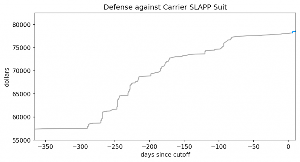
The last year of donations, for the lawsuit fundraiser.

The donations seem to arrive in bursts, but there have been two quiet portions. One is thanks to the current pandemic, and the other was during last year’s late spring/early summer. It’s hard to tell what the donation rate is just by eye-ball, though. We need to smooth this out via a model.
The simplest such model is linear regression, aka. fitting a line. We want to incorporate uncertainty into the mix, which means a Bayesian fit. Now, what MCMC engine to use, hmmm…. emcee is my overall favourite, but I’m much too reliant on it. I’ve used PyMC3 a few times with success, but recently it’s been acting flaky. Time to pull out the big guns: Stan. I’ve been avoiding it because pystan‘s compilation times drove me nuts, but all the cool kids have switched to cmdstanpy when I looked away. Let’s give that a whirl.

(Click here to show the code)
CPU times: user 5.33 ms, sys: 7.33 ms, total: 12.7 ms
Wall time: 421 ms
CmdStan installed.

We can’t fit to the entire three-year time sequence, that just wouldn’t be fair given the recent slump in donations. How about the last six months? That covers both a few donation burts and a flat period, so it’s more in line with what we’d expect in future.

(Click here to show the code)
There were 117 donations over the last six months.

With the data prepped, we can shift to building the linear model.

(Click here to show the code)

I could have just gone with Stan’s basic model, but flat priors aren’t my style. My preferred prior for the slope is the inverse tangent, as it compensates for the tendency of large slope values to “bunch up” on one another. Stan doesn’t offer it by default, but the Cauchy distribution isn’t too far off.

We’d like the standard deviation to skew towards smaller values. It naturally tends to minimize itself when maximizing the likelihood, but an explicit skew will encourage this process along. Gelman and the Stan crew are drifting towards normal priors, but I still like a Cauchy prior for its weird properties.

Normally I’d plunk the Gaussian distribution in to handle divergence from the deterministic model, but I hear using Student’s T instead will cut down the influence of outliers. Thomas Wiecki recommends one degree of freedom, but Gelman and co. find that it leads to poor convergence in some cases. They recommend somewhere between three and seven degrees of freedom, but skew towards three, so I’ll go with the flow here.

The y-intercept could land pretty much anywhere, making its prior difficult to figure out. Yes, I’ve adjusted the time axis so that the last donation is at time zero, but the recent flat portion pretty much guarantees the y-intercept will be higher than the current amount of funds. The traditional approach is to use a flat prior for the intercept, and I can’t think of a good reason to ditch that.

Not convinced I picked good priors? That’s cool, there should be enough data here that the priors have minimal influence anyway. Moving on, let’s see how long compilation takes.

(Click here to show the code)
CPU times: user 4.91 ms, sys: 5.3 ms, total: 10.2 ms
Wall time: 20.2 s

This is one area where emcee really shines: as a pure python library, it has zero compilation time. Both PyMC3 and Stan need some time to fire up an external compiler, which adds overhead. Twenty seconds isn’t too bad, though, especially if it leads to quick sampling times.

(Click here to show the code)
CPU times: user 14.7 ms, sys: 24.7 ms, total: 39.4 ms
Wall time: 829 ms

And it does! emcee can be pretty zippy for a simple linear regression, but Stan is in another class altogether. PyMC3 floats somewhere between the two, in my experience.

Another great feature of Stan are the built-in diagnostics. These are really handy for confirming the posterior converged, and if not it can give you tips on what’s wrong with the model.

(Click here to show the code)
Processing csv files: /tmp/tmpyfx91ua9/linear_regression-202005262238-1-e393mc6t.csv, /tmp/tmpyfx91ua9/linear_regression-202005262238-2-8u_r8umk.csv, /tmp/tmpyfx91ua9/linear_regression-202005262238-3-m36dbylo.csv, /tmp/tmpyfx91ua9/linear_regression-202005262238-4-hxjnszfe.csv

Checking sampler transitions treedepth.
Treedepth satisfactory for all transitions.

Checking sampler transitions for divergences.
No divergent transitions found.

Checking E-BFMI - sampler transitions HMC potential energy.
E-BFMI satisfactory for all transitions.

Effective sample size satisfactory.

Split R-hat values satisfactory all parameters.

Processing complete, no problems detected.

The odds of a simple model with plenty of datapoints going sideways are pretty small, so this is another non-surprise. Enough waiting, though, let’s see the fit in action. First, we need to extract the posterior from the stored variables …

(Click here to show the code)
There are 256 samples in the posterior.

… and now free of its prison, we can plot the posterior against the original data. I’ll narrow the time window slightly, to make it easier to focus on the fit.

(Click here to show the code)

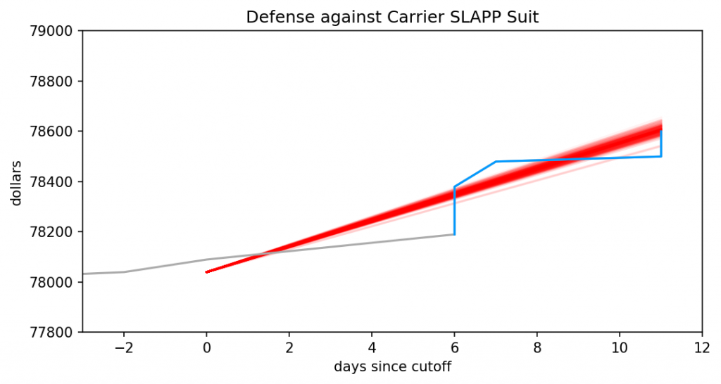
The same graph as before, but now slightly zoomed in on and with trendlines visible.

Looks like a decent fit to me, so we can start using it to answer a few questions. How much money is flowing into the fund each day, on average? How many years will it be until all those legal bills are paid off? Since humans aren’t good at counting in years, let’s also translate that number into a specific date.

(Click here to show the code)
mean/std/median slope = $51.62/1.65/51.76 per day

mean/std/median years to pay off the legal fees, relative to 2020-05-25 12:36:39-05:00 =
	1.962/0.063/1.955

mean/median estimate for paying off debt =
	2022-05-12 07:49:55.274942-05:00 / 2022-05-09 13:57:13.461426-05:00

Mid-May 2022, eh? That’s… not ideal. How much time can we shave off, if we increase the donation rate? Let’s play out a few scenarios.

(Click here to show the code)
median estimate for paying off debt, increasing rate by   1% = 2022-05-02 17:16:37.476652800
median estimate for paying off debt, increasing rate by   3% = 2022-04-18 23:48:28.185868800
median estimate for paying off debt, increasing rate by  10% = 2022-03-05 21:00:48.510403200
median estimate for paying off debt, increasing rate by  30% = 2021-11-26 00:10:56.277984
median estimate for paying off debt, increasing rate by 100% = 2021-05-17 18:16:56.230752

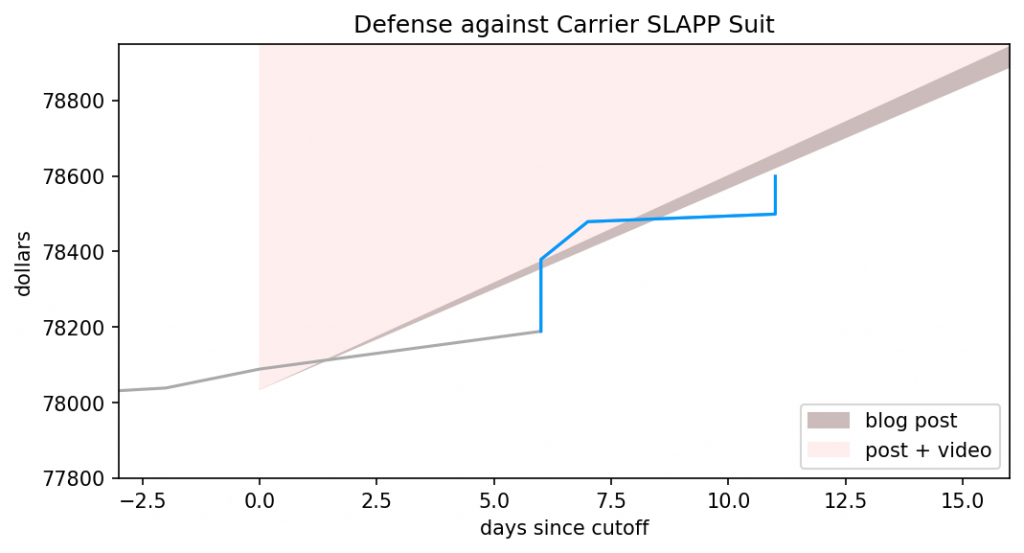
Bumping up the donation rate by one percent is pitiful. A three percent increase will almost shave off a month, which is just barely worthwhile, and a ten percent increase will roll the date forward by two. Those sound like good starting points, so let’s make them official: increase the current donation rate by three percent, and I’ll start pumping out the aforementioned blog posts on Bayesian statistics. Manage to increase it by 10%, and I’ll also record them as videos.

As implied, I don’t intend to keep the same rate throughout this entire process. If you surprise me with your generosity, I’ll bump up the rate. By the same token, though, if we go through a dry spell I’ll decrease the rate so the targets are easier to hit. My goal is to have at least a 50% success rate on that lower bar. Wouldn’t that make it impossible to hit the video target? Remember, though, it’ll take some time to determine the success rate. That lag should make it possible to blow past the target, and by the time this becomes an issue I’ll have thought of a better fix.

Ah, but over what timeframe should this rate increase? We could easily blow past the three percent target if someone donates a hundred bucks tomorrow, after all, and it’s no fair to announce this and hope your wallets are ready to go in an instant. How about… sixteen days. You’ve got sixteen days to hit one of those rate targets. That’s a nice round number, for a computer scientist, and it should (hopefully!) give me just enough time to whip up the first post. What does that goal translate to, in absolute numbers?

(Click here to show the code)
a   3% increase over 16 days translates to $851.69 + $78039.00 = $78890.69

Right, if you want those blog posts to start flowing you’ve got to get that fundraiser total to $78,890.69 before June 12th. As for the video…

(Click here to show the code)
a  10% increase over 16 days translates to $909.57 + $78039.00 = $78948.57

… you’ve got to hit $78,948.57 by the same date.

Ready? Set? Get donating!

It’s Payback Time

I’m back! Yay! Sorry about all that, but my workload was just ridiculous. Things should be a lot more slack for the next few months, so it’s time I got back blogging. This also means I can finally put into action something I’ve been sitting on for months.

Richard Carrier has been a sore spot for me. He was one of the reasons I got interested in Bayesian statistics, and for a while there I thought he was a cool progressive. Alas, when it was revealed he was instead a vindictive creepy asshole, it shook me a bit. I promised myself I’d help out somehow, but I’d already done the obsessive analysis thing and in hindsight I’m not convinced it did more good than harm. I was at a loss for what I could do, beyond sharing links to the fundraiser.

Now, I think I know. The lawsuits may be long over, thanks to Carrier coincidentally dropping them at roughly the same time he came under threat of a counter-suit, but the legal bill are still there and not going away anytime soon. Worse, with the removal of the threat people are starting to forget about those debts. There have been only five donations this month, and four in April. It’s time to bring a little attention back that way.

One nasty side-effect of Carrier’s lawsuits is that Bayesian statistics has become a punchline in the atheist/skeptic community. The reasoning is understandable, if flawed: Carrier is a crank, he promotes Bayesian statistics, ergo Bayesian statistics must be the tool of crackpots. This has been surreal for me to witness, as Bayes has become a critical tool in my kit over the last three years. I suppose I could survive without it, if I had to, but every alternative I’m aware of is worse. I’m not the only one in this camp, either.

Following the emergence of a novel coronavirus (SARS-CoV-2) and its spread outside of China, Europe is now experiencing large epidemics. In response, many European countries have implemented unprecedented non-pharmaceutical interventions including case isolation, the closure of schools and universities, banning of mass gatherings and/or public events, and most recently, widescale social distancing including local and national lockdowns. In this report, we use a semi-mechanistic Bayesian hierarchical model to attempt to infer the impact of these interventions across 11 European countries.

Flaxman, Seth, Swapnil Mishra, Axel Gandy, H Juliette T Unwin, Helen Coupland, Thomas A Mellan, Tresnia Berah, et al. “Estimating the Number of Infections and the Impact of Non- Pharmaceutical Interventions on COVID-19 in 11 European Countries,” 2020, 35.

In estimating time intervals between symptom onset and outcome, it was necessary to account for the fact that, during a growing epidemic, a higher proportion of the cases will have been infected recently (…). Therefore, we re-parameterised a gamma model to account for exponential growth using a growth rate of 0·14 per day, obtained from the early case onset data (…). Using Bayesian methods, we fitted gamma distributions to the data on time from onset to death and onset to recovery, conditional on having observed the final outcome.

Verity, Robert, Lucy C. Okell, Ilaria Dorigatti, Peter Winskill, Charles Whittaker, Natsuko Imai, Gina Cuomo-Dannenburg, et al. “Estimates of the Severity of Coronavirus Disease 2019: A Model-Based Analysis.” The Lancet Infectious Diseases 0, no. 0 (March 30, 2020). https://doi.org/10.1016/S1473-3099(20)30243-7.

we used Bayesian methods to infer parameter estimates and obtain credible intervals.

Linton, Natalie M., Tetsuro Kobayashi, Yichi Yang, Katsuma Hayashi, Andrei R. Akhmetzhanov, Sung-mok Jung, Baoyin Yuan, Ryo Kinoshita, and Hiroshi Nishiura. “Incubation Period and Other Epidemiological Characteristics of 2019 Novel Coronavirus Infections with Right Truncation: A Statistical Analysis of Publicly Available Case Data.” Journal of Clinical Medicine 9, no. 2 (February 2020): 538. https://doi.org/10.3390/jcm9020538.

A significant chunk of our understanding of COVID-19 depends on Bayesian statistics. I’ll go further and argue that you cannot fully understand this pandemic without it. And yet thanks to Richard Carrier, the atheist/skeptic community is primed to dismiss Bayesian statistics.

So let’s catch two stones with one bird. If enough people donate to this fundraiser, I’ll start blogging a course on Bayesian statistics. I think I’ve got a novel angle on the subject, one that’s easier to slip into than my 201-level stuff and yet more rigorous. If y’all really start tossing in the funds, I’ll make it a video series. Yes yes, there’s a pandemic and potential global depression going on, but that just means I’ll work for cheap! I’ll release the milestones and course outline over the next few days, but there’s no harm in an early start.

Help me help the people Richard Carrier hurt. I’ll try to make it worth your while.

Dear Bob Carpenter,

Hello! I’ve been a fan of your work for some time. While I’ve used emcee more and currently use a lot of PyMC3, I love the layout of Stan‘s language and often find myself missing it.

But there’s no contradiction between being a fan and critiquing your work. And one of your recent blog posts left me scratching my head.

Suppose I want to estimate my chances of winning the lottery by buying a ticket every day. That is, I want to do a pure Monte Carlo estimate of my probability of winning. How long will it take before I have an estimate that’s within 10% of the true value?

This one’s pretty easy to set up, thanks to conjugate priors. The Beta distribution models our credibility of the odds of success from a Bernoulli process. If our prior belief is represented by the parameter pair \((\alpha_\text{prior},\beta_\text{prior})\), and we win \(w\) times over \(n\) trials, our posterior belief in the odds of us winning the lottery, \(p\), is

$$ \begin{align}
\alpha_\text{posterior} &= \alpha_\text{prior} + w, \\
\beta_\text{posterior} &= \beta_\text{prior} + n – w
\end{align} $$

You make it pretty clear that by “lottery” you mean the traditional kind, with a big payout that your highly unlikely to win, so \(w \approx 0\). But in the process you make things much more confusing.

There’s a big NY state lottery for which there is a 1 in 300M chance of winning the jackpot. Back of the envelope, to get an estimate within 10% of the true value of 1/300M will take many millions of years.

“Many millions of years,” when we’re “buying a ticket every day?” That can’t be right. The mean of the Beta distribution is

$$ \begin{equation}
\mathbb{E}[Beta(\alpha_\text{posterior},\beta_\text{posterior})] = \frac{\alpha_\text{posterior}}{\alpha_\text{posterior} + \beta_\text{posterior}}
\end{equation} $$

So if we’re trying to get that within 10% of zero, and \(w = 0\), we can write

$$ \begin{align}
\frac{\alpha_\text{prior}}{\alpha_\text{prior} + \beta_\text{prior} + n} &< \frac{1}{10} \\
10 \alpha_\text{prior} &< \alpha_\text{prior} + \beta_\text{prior} + n \\
9 \alpha_\text{prior} – \beta_\text{prior} &< n
\end{align} $$

If we plug in a sensible-if-improper subjective prior like \(\alpha_\text{prior} = 0, \beta_\text{prior} = 1\), then we don’t even need to purchase a single ticket. If we insist on an “objective” prior like Jeffrey’s, then we need to purchase five tickets. If for whatever reason we foolishly insist on the Bayes/Laplace prior, we need nine tickets. Even at our most pessimistic, we need less than a fortnight (or, if you prefer, much less than a Fortnite season). If we switch to the maximal likelihood instead of the mean, the situation gets worse.

$$ \begin{align}
\text{Mode}[Beta(\alpha_\text{posterior},\beta_\text{posterior})] &= \frac{\alpha_\text{posterior} – 1}{\alpha_\text{posterior} + \beta_\text{posterior} – 2} \\
\frac{\alpha_\text{prior} – 1}{\alpha_\text{prior} + \beta_\text{prior} + n – 2} &< \frac{1}{10} \\
9\alpha_\text{prior} – \beta_\text{prior} – 8 &< n
\end{align} $$

Now Jeffrey’s prior doesn’t require us to purchase a ticket, and even that awful Bayes/Laplace prior needs just one purchase. I can’t see how you get millions of years out of that scenario.

In the Interval

Maybe you meant a different scenario, though. We often use credible intervals to make decisions, so maybe you meant that the entire interval has to pass below the 0.1 mark? This introduces another variable, the width of the credible interval. Most people use two standard deviations or thereabouts, but I and a few others prefer a single standard deviation. Let’s just go with the higher bar, and start hacking away at the variance of the Beta distribution.

$$ \begin{align}
\text{var}[Beta(\alpha_\text{posterior},\beta_\text{posterior})] &= \frac{\alpha_\text{posterior}\beta_\text{posterior}}{(\alpha_\text{posterior} + \beta_\text{posterior})^2(\alpha_\text{posterior} + \beta_\text{posterior} + 2)} \\
\sigma[Beta(\alpha_\text{posterior},\beta_\text{posterior})] &= \sqrt{\frac{\alpha_\text{prior}(\beta_\text{prior} + n)}{(\alpha_\text{prior} + \beta_\text{prior} + n)^2(\alpha_\text{prior} + \beta_\text{prior} + n + 2)}} \\
\frac{\alpha_\text{prior}}{\alpha_\text{prior} + \beta_\text{prior} + n} + \frac{2}{\alpha_\text{prior} + \beta_\text{prior} + n} \sqrt{\frac{\alpha_\text{prior}(\beta_\text{prior} + n)}{\alpha_\text{prior} + \beta_\text{prior} + n + 2}} &< \frac{1}{10}
\end{align} $$

Our improper subjective prior still requires zero ticket purchases, as \(\alpha_\text{prior} = 0\) wipes out the entire mess. For Jeffrey’s prior, we find

$$ \begin{equation}
\frac{\frac{1}{2}}{n + 1} + \frac{2}{n + 1} \sqrt{\frac{1}{2}\frac{n + \frac 1 2}{n + 3}} < \frac{1}{10},
\end{equation} $$

which needs 18 ticket purchases according to Wolfram Alpha. The awful Bayes/Laplace prior can almost get away with 27 tickets, but not quite. Both of those stretch the meaning of “back of the envelope,” but you can get the answer via a calculator and some trial-and-error.

I used the term “hacking” for a reason, though. That variance formula is only accurate when \(p \approx \frac 1 2\) or \(n\) is large, and neither is true in this scenario. We’re likely underestimating the number of tickets we’d need to buy. To get an accurate answer, we need to integrate the Beta distribution.

$$ \begin{align}
\int_{p=0}^{\frac{1}{10}} \frac{\Gamma(\alpha_\text{posterior} + \beta_\text{posterior})}{\Gamma(\alpha_\text{posterior})\Gamma(\beta_\text{posterior})} p^{\alpha_\text{posterior} – 1} (1-p)^{\beta_\text{posterior} – 1} > \frac{39}{40} \\
40 \frac{\Gamma(\alpha_\text{prior} + \beta_\text{prior} + n)}{\Gamma(\alpha_\text{prior})\Gamma(\beta_\text{prior} + n)} \int_{p=0}^{\frac{1}{10}} p^{\alpha_\text{prior} – 1} (1-p)^{\beta_\text{prior} + n – 1} > 39
\end{align} $$

Awful, but at least for our subjective prior it’s trivial to evaluate. \(\text{Beta}(0,n+1)\) is a Dirac delta at \(p = 0\), so 100% of the integral is below 0.1 and we still don’t need to purchase a single ticket. Fortunately for both the Jeffrey’s and Bayes/Laplace prior, my “envelope” is a Jupyter notebook.

(Click here to show the code)

A graph of the integrals for varying n. Jeffrey's prior crosses the 0.975 threshold at 25, while Bayes/Laplace waits until 36.

Those numbers did go up by a non-trivial amount, but we’re still nowhere near “many millions of years,” even if Fortnite’s last season felt that long.

Maybe you meant some scenario where the credible interval overlaps \(p = 0\)? With proper priors, that never happens; the lower part of the credible interval always leaves room for some extremely small values of \(p\), and thus never actually equals 0. My sensible improper prior has both ends of the interval equal to zero and thus as long as \(w = 0\) it will always overlap \(p = 0\).

Expecting Something?

I think I can find a scenario where you’re right, but I also bet you’re sick of me calling \((0,1)\) a “sensible” subjective prior. Hope you don’t mind if I take a quick detour to the last question in that blog post, which should explain how a Dirac delta can be sensible.

How long would it take to convince yourself that playing the lottery has an expected negative return if tickets cost $1, there’s a 1/300M chance of winning, and the payout is $100M?

Let’s say the payout if you win is \(W\) dollars, and the cost of a ticket is \(T\). Then your expected earnings at any moment is an integral of a multiple of the entire Beta posterior.
$$ \begin{equation}
\mathbb{E}(\text{Lottery}_{W}) = \int_{p=0}^1 \frac{\Gamma(\alpha_\text{posterior} + \beta_\text{posterior})}{\Gamma(\alpha_\text{posterior})\Gamma(\beta_\text{posterior})} p^{\alpha_\text{posterior} – 1} (1-p)^{\beta_\text{posterior} – 1} p W < T
\end{equation} $$

I’m pretty confident you can see why that’s a back-of-the-envelope calculation, but this is a public letter and I’m also sure some of those readers just fainted. Let me detour from the detour to assure them that, yes, this is actually a pretty simple calculation. They’ve already seen that multiplicative constants can be yanked out of the integral, but I’m not sure they realized that if

$$ \begin{equation}
\int_{p=0}^1 \frac{\Gamma(\alpha + \beta)}{\Gamma(\alpha)\Gamma(\beta)} p^{\alpha – 1} (1-p)^{\beta – 1} = 1,
\end{equation} $$

then thanks to the multiplicative constant rule it must be true that

$$ \begin{equation}
\int_{p=0}^1 p^{\alpha – 1} (1-p)^{\beta – 1} = \frac{\Gamma(\alpha)\Gamma(\beta)}{\Gamma(\alpha + \beta)}
\end{equation} $$

They may also be unaware that the Gamma function is an analytic continuity of the factorial. I say “an” because there’s an infinite number of functions that also qualify. To be considered a “good” analytic continuity the Gamma function must also duplicate another property of the factorial, that \((a + 1)! = (a + 1)(a!)\) for all valid \(a\). Or, put another way, it must be true that

$$ \begin{equation}
\frac{\Gamma(a + 1)}{\Gamma(a)} = a + 1, a > 0
\end{equation} $$

Fortunately for me, the Gamma function is a good analytic continuity, perhaps even the best. This allows me to chop that integral down to size.

$$ \begin{align}
W \frac{\Gamma(\alpha_\text{prior} + \beta_\text{prior} + n)}{\Gamma(\alpha_\text{prior})\Gamma(\beta_\text{prior} + n)} \int_{p=0}^1 p^{\alpha_\text{prior} – 1} (1-p)^{\beta_\text{prior} + n – 1} p &< T \\
\int_{p=0}^1 p^{\alpha_\text{prior} – 1} (1-p)^{\beta_\text{prior} + n – 1} p &= \int_{p=0}^1 p^{\alpha_\text{prior}} (1-p)^{\beta_\text{prior} + n – 1} \\
\int_{p=0}^1 p^{\alpha_\text{prior}} (1-p)^{\beta_\text{prior} + n – 1} &= \frac{\Gamma(\alpha_\text{prior} + 1)\Gamma(\beta_\text{prior} + n)}{\Gamma(\alpha_\text{prior} + \beta_\text{prior} + n + 1)} \\
W \frac{\Gamma(\alpha_\text{prior} + \beta_\text{prior} + n)}{\Gamma(\alpha_\text{prior})\Gamma(\beta_\text{prior} + n)} \frac{\Gamma(\alpha_\text{prior} + 1)\Gamma(\beta_\text{prior} + n)}{\Gamma(\alpha_\text{prior} + \beta_\text{prior} + n + 1)} &< T \\
W \frac{\Gamma(\alpha_\text{prior} + \beta_\text{prior} + n) \Gamma(\alpha_\text{prior} + 1)}{\Gamma(\alpha_\text{prior} + \beta_\text{prior} + n + 1) \Gamma(\alpha_\text{prior})} &< T \\
W \frac{\alpha_\text{prior} + 1}{\alpha_\text{prior} + \beta_\text{prior} + n + 1} &< T \\
\frac{W}{T}(\alpha_\text{prior} + 1) – \alpha_\text{prior} – \beta_\text{prior} – 1 &< n
\end{align} $$

Mmmm, that was satisfying. Anyway, for Jeffrey’s prior you need to purchase \(n > 149,999,998\) tickets to be convinced this lottery isn’t worth investing in, while the Bayes/Laplace prior argues for \(n > 199,999,997\) purchases. Plug my subjective prior in, and you’d need to purchase \(n > 99,999,998\) tickets.

That’s optimal, assuming we know little about the odds of winning this lottery. The number of tickets we need to purchase is controlled by our prior. Since \(W \gg T\), our best bet to minimize the number of tickets we need to purchase is to minimize \(\alpha_\text{prior}\). Unfortunately, the lowest we can go is \(\alpha_\text{prior} = 0\). Almost all the “objective” priors I know of have it larger, and thus ask that you sink more money into the lottery than the prize is worth. That doesn’t sit well with our intuition. The sole exception is the Haldane prior of (0,0), which argues for \(n > 99,999,999\) and thus asks you to spend exactly as much as the prize-winnings. By stating \(\beta_\text{prior} = 1\), my prior manages to shave off one ticket purchase.

Another prior that increases \(\beta_\text{prior}\) further will shave off further purchases, but so far we’ve only considered the case where \(w = 0\). What if we sink money into this lottery, and happen to win before hitting our limit? The subjective prior of \((0,1)\) after \(n\) losses becomes equivalent to the Bayes/Laplace prior of \((1,1)\) after \(n-1\) losses. Our assumption that \(p \approx 0\) has been proven wrong, so the next best choice is to make no assumptions about \(p\). At the same time, we’ve seen \(n\) losses and we’d be foolish to discard that information entirely. A subjective prior with \(\beta_\text{prior} > 1\) wouldn’t transform in this manner, while one with \(\beta_\text{prior} < 1\) would be biased towards winning the lottery relative to the Bayes/Laplace prior.

My subjective prior argues you shouldn’t play the lottery, which matches the reality that almost all lotteries pay out less than they take in, but if you insist on participating it will minimize your losses while still responding well to an unexpected win. It lives up to the hype.

However, there is one way to beat it. You mentioned in your post that the odds of winning this lottery are one in 300 million. We’re not supposed to incorporate that into our math, it’s just a measuring stick to use against the values we churn out, but what if we constructed a prior around it anyway? This prior should have a mean of one in 300 million, and the \(p = 0\) case should have zero likelihood. The best match is \((1+\epsilon, 299999999\cdot(1+\epsilon))\), where \(\epsilon\) is a small number, and when we take a limit …

$$ \begin{equation}
\lim_{\epsilon \to 0^{+}} \frac{100,000,000}{1}(2 + \epsilon) – 299,999,999 \epsilon – 300,000,000 = -100,000,000 < n
\end{equation} $$

… we find the only winning move is not to play. There’s no Dirac deltas here, either, so unlike my subjective prior it’s credible interval is one-dimensional. Eliminating the \(p = 0\) case runs contrary to our intuition, however. A newborn that purchased a ticket every day of its life until it died on its 80th birthday has a 99.99% chance of never holding a winning ticket. \(p = 0\) is always an option when you live a finite amount of time.

The problem with this new prior is that it’s incredibly strong. If we didn’t have the true odds of winning in our back pocket, we could quite fairly be accused of putting our thumb on the scales. We can water down \((1,299999999)\) by dividing both \(\alpha_\text{prior}\) and \(\beta_\text{prior}\) by a constant value. This maintains the mean of the Beta distribution, and while the \(p = 0\) case now has non-zero credence I’ve shown that’s no big deal. Pick the appropriate constant value and we get something like \((\epsilon,1)\), where \(\epsilon\) is a small positive value. Quite literally, that’s within epsilon of the subjective prior I’ve been hyping!

Enter Frequentism

So far, the only back-of-the-envelope calculations I’ve done that argued for millions of ticket purchases involved the expected value, but that was only because we used weak priors that are a poor match for reality. I believe in the principle of charity, though, and I can see a scenario where a back-of-the-envelope calculation does demand millions of purchases.

But to do so, I’ve got to hop the fence and become a frequentist.

If you haven’t read The Theory That Would Not Die, you’re missing out. Sharon Bertsch McGrayne mentions one anecdote about the RAND Corporation’s attempts to calculate the odds of a nuclear weapon accidentally detonating back in the 1950’s. No frequentist statistician would touch it with a twenty-foot pole, but not because they were worried about getting the math wrong. The problem was the math. As the eventually-published report states:

The usual way of estimating the probability of an accident in a given situation is to rely on observations of past accidents. This approach is used in the Air Force, for example, by the Directory of Flight Safety Research to estimate the probability per flying hour of an aircraft accident. In cases of of newly introduced aircraft types for which there are no accident statistics, past experience of similar types is used by analogy.

Such an approach is not possible in a field where this is no record of past accidents. After more than a decade of handling nuclear weapons, no unauthorized detonation has occurred. Furthermore, one cannot find a satisfactory analogy to the complicated chain of events that would have to precede an unauthorized nuclear detonation. (…) Hence we are left with the banal observation that zero accidents have occurred. On this basis the maximal likelihood estimate of the probability of an accident in any future exposure turns out to be zero.

For the lottery scenario, a frequentist wouldn’t reach for the Beta distribution but instead the Binomial. Given \(n\) trials of a Bernoulli process with probability \(p\) of success, the expected number of successes observed is

$$ \begin{equation}
\bar w = n p
\end{equation} $$

We can convert that to a maximal likelihood estimate by dividing the actual number of observed successes by \(n\).

$$ \begin{equation}
\hat p = \frac{w}{n}
\end{equation} $$

In many ways this estimate can be considered optimal, as it is both unbiased and has the least variance of all other estimators. Thanks to the Central Limit Theorem, the Binomial distribution will approximate a Gaussian distribution to arbitrary degree as we increase \(n\), which allows us to apply the analysis from the latter to the former. So we can use our maximal likelihood estimate \(\hat p\) to calculate the standard error of that estimate.

$$ \begin{equation}
\text{SEM}[\hat p] = \sqrt{ \frac{\hat p(1- \hat p)}{n} }
\end{equation} $$

Ah, but what if \(w = 0\)? It follows that \(\hat p = 0\), but this also means that \(\text{SEM}[\hat p] = 0\). There’s no variance in our estimate? That can’t be right. If we approach this from another angle, plugging \(w = 0\) into the Binomial distribution, it reduces to

$$ \begin{equation}
\text{Binomial}(w | n,p) = \frac{n!}{w!(n-w)!} p^w (1-p)^{n-w} = (1-p)^n
\end{equation} $$

The maximal likelihood of this Binomial is indeed \(p = 0\), but it doesn’t resemble a Dirac delta at all.

(Click here to show the code)

The binomial distribution for k=0, n=25. It has a peak at p=0, and drops off to zero at p=1.

Shouldn’t there be some sort of variance there? What’s going wrong?

We got a taste of this on the Bayesian side of the fence. Using the stock formula for the variance of the Beta distribution underestimated the true value, because the stock formula assumed \(p \approx \frac 1 2\) or a large \(n\). When we assume we have a near-infinite amount of data, we can take all sorts of computational shortcuts that make our life easier. One look at the Binomial’s mean, however, tells us that we can drown out the effects of a large \(n\) with a small value of \(p\). And, just as with the odds of a nuclear bomb accident, we already know \(p\) is very, very small. That isn’t fatal on its own, as you correctly point out.

With the lottery, if you run a few hundred draws, your estimate is almost certainly going to be exactly zero. Did we break the [*Central Limit Theorem*]? Nope. Zero has the right absolute error properties. It’s within 1/300M of the true answer after all!

The problem comes when we apply the Central Limit Theorem and use a Gaussian approximation to generate a confidence or credible interval for that maximal likelihood estimate. As both the math and graph show, though, the probability distribution isn’t well-described by a Gaussian distribution. This isn’t much of a problem on the Bayesian side of the fence, as I can juggle multiple priors and switch to integration for small values of \(n\). Frequentism, however, is dependent on the Central Limit Theorem and thus assumes \(n\) is sufficiently large. This is baked right into the definitions: a p-value is the fraction of times you calculate a test metric equal to or more extreme than the current one assuming the null hypothesis is true and an infinite number of equivalent trials of the same random process, while confidence intervals are a range of parameter values such that when we repeat the maximal likelihood estimate on an infinite number of equivalent trials the estimates will fall in that range more often than a fraction of our choosing. Frequentist statisticians are stuck with the math telling them that \(p = 0\) with absolute certainty, which conflicts with our intuitive understanding.

For a frequentist, there appears to be only one way out of this trap: witness a nuclear bomb accident. Once \(w > 0\), the math starts returning values that better match intuition. Likewise with the lottery scenario, the only way for a frequentist to get an estimate of \(p\) that comes close to their intuition is to purchase tickets until they win at least once.

This scenario does indeed take “many millions of years.” It’s strange to find you taking a frequentist world-view, though, when you’re clearly a Bayesian. By straddling the fence you wind up in a world of hurt. For instance, you state this:

Did we break the [*Central Limit Theorem*]? Nope. Zero has the right absolute error properties. It’s within 1/300M of the true answer after all! But it has terrible relative error probabilities; it’s relative error after a lifetime of playing the lottery is basically infinity.

A true frequentist would have been fine asserting the probability of a nuclear bomb accident is zero. Why? Because \(\text{SEM}[\hat p = 0]\) is actually a very good confidence interval. If we’re going for two sigmas, then our confidence interval should contain the maximal likelihood we’ve calculated at least 95% of the time. Let’s say our sample sizes are \(n = 36\), the worst-case result from Bayesian statistics. If the true odds of winning the lottery are 1 in 300 million, then the odds of calculating a maximal likelihood of \(p = 0\) is

(Click here to show the code)
p( MLE(hat p) = 0 ) =  0.999999880000007

About 99.99999% of the time, then, the confidence interval of \(0 \leq \hat p \leq 0\) will be correct. That’s substantially better than 95%! Nothing’s broken here, frequentism is working exactly as intended.

I bet you think I’ve screwed up the definition of confidence intervals. I’m afraid not, I’ve double-checked my interpretation by heading back to the source, Jerzy Neyman. He, more than any other person, is responsible for pioneering the frequentist confidence interval.

We can then tell the practical statistician that whenever he is certain that the form of the probability law of the X’s is given by the function? \(p(E|\theta_1, \theta_2, \dots \theta_l,)\) which served to determine \(\underline{\theta}(E)\) and \(\bar \theta(E)\) [the lower and upper bounds of the confidence interval], he may estimate \(\theta_1\) by making the following three steps: (a) he must perform the random experiment and observe the particular values \(x_1, x_2, \dots x_n\) of the X’s; (b) he must use these values to calculate the corresponding values of \(\underline{\theta}(E)\) and \(\bar \theta(E)\); and (c) he must state that \(\underline{\theta}(E) < \theta_1^o < \bar \theta(E)\), where \(\theta_1^o\) denotes the true value of \(\theta_1\). How can this recommendation be justified?

[Neyman keeps alternating between \(\underline{\theta}(E) \leq \theta_1^o \leq \bar \theta(E)\) and \(\underline{\theta}(E) < \theta_1^o < \bar \theta(E)\) throughout this paper, so presumably both forms are A-OK.]

The justification lies in the character of probabilities as used here, and in the law of great numbers. According to this empirical law, which has been confirmed by numerous experiments, whenever we frequently and independently repeat a random experiment with a constant probability, \(\alpha\), of a certain result, A, then the relative frequency of the occurrence of this result approaches \(\alpha\). Now the three steps (a), (b), and (c) recommended to the practical statistician represent a random experiment which may result in a correct statement concerning the value of \(\theta_1\). This result may be denoted by A, and if the calculations leading to the functions \(\underline{\theta}(E)\) and \(\bar \theta(E)\) are correct, the probability of A will be constantly equal to \(\alpha\). In fact, the statement (c) concerning the value of \(\theta_1\) is only correct when \(\underline{\theta}(E)\) falls below \(\theta_1^o\) and \(\bar \theta(E)\), above \(\theta_1^o\), and the probability of this is equal to \(\alpha\) whenever \(\theta_1^o\) the true value of \(\theta_1\). It follows that if the practical statistician applies permanently the rules (a), (b) and (c) for purposes of estimating the value of the parameter \(\theta_1\) in the long run he will be correct in about 99 per cent of all cases. []

It will be noticed that in the above description the probability statements refer to the problems of estimation with which the statistician will be concerned in the future. In fact, I have repeatedly stated that the frequency of correct results tend to \(\alpha\). [Footnote: This, of course, is subject to restriction that the X’s considered will follow the probability law assumed.] Consider now the case when a sample, E’, is already drawn and the calculations have given, say, \(\underline{\theta}(E’)\) = 1 and \(\bar \theta(E’)\) = 2. Can we say that in this particular case the probability of the true value of \(\theta_1\) falling between 1 and 2 is equal to \(\alpha\)?

The answer is obviously in the negative. The parameter \(\theta_1\) is an unknown constant and no probability statement concerning its value may be made, that is except for the hypothetical and trivial ones … which we have decided not to consider.

Neyman, Jerzy. “X — outline of a theory of statistical estimation based on the classical theory of probability.” Philosophical Transactions of the Royal Society of London. Series A, Mathematical and Physical Sciences 236.767 (1937): 348-349.

If there was any further doubt, it’s erased when Neyman goes on to analogize scientific measurements to a game of roulette. Just as the knowing where the ball landed doesn’t tell us anything about where the gamblers placed their bets, “once the sample \(E’\) is drawn and the values of \(\underline{\theta}(E’)\) and \(\bar \theta(E’)\) determined, the calculus of probability adopted here is helpless to provide answer to the question of what is the true value of \(\theta_1\).” (pg. 350)

If a confidence interval doesn’t tell us anything about where the true parameter value lies, then its only value must come from being an estimator of long-term behaviour. And as I showed before, \(\text{SEM}[\hat p = 0]\) estimates the maximal likelihood from repeating the experiment extremely well. It is derived from the long-term behaviour of the Binomial distribution, which is the correct distribution to describe this situation within frequentism. \(\text{SEM}[\hat p = 0]\) fits Neyman’s definition of a confidence interval perfectly, and thus generates a valid frequentist confidence interval. On the Bayesian side, I’ve spilled a substantial number of photons to convince you that a Dirac delta prior is a good choice, and that prior also generates zero-width credence intervals. If it worked over there, why can’t it also work over here?

This is Jayne’s Truncated Interval all over again. The rules of frequentism don’t work the way we intuit, which normally isn’t a problem because the Central Limit Theorem massages the data enough to align frequentism and intuition. Here, though, we’ve stumbled on a corner case where \(p = 0\) with absolute certainty and \(p \neq 0\) with tight error bars are both correct conclusions under the rules of frequentism. RAND Corporation should not have had any difficulty finding a frequentist willing to calculate the odds of a nuclear bomb accident, because they could have scribbled out one formula on an envelope and concluded such accidents were impossible.

And yet, faced with two contradictory answers or unaware the contradiction exists, frequentists side with intuition and reject the rules of their own statistical system. They strike off the \(p = 0\) answer, leaving only the case where \(p \ne 0\) and \(w > 0\). Since reality currently insists that \(w = 0\), they’re prevented from coming to any conclusion. The same reasoning leads to the “many millions of years” of ticket purchases that you argued was the true back-of-the-envelope conclusion. To break out of this rut, RAND Corporation was forced to abandon frequentism and instead get their estimate via Bayesian statistics.

On this basis the maximal likelihood estimate of the probability of an accident in any future exposure turns out to be zero. Obviously we cannot rest content with this finding. []

… we can use the following idea: in an operation where an accident seems to be possible on technical grounds, our assurance that this operation will not lead to an accident in the future increases with the number of times this operation has been carried out safely, and decreases with the number of times it will be carried out in the future. Statistically speaking, this simple common sense idea is based on the notion that there is an a priori distribution of the probability of an accident in a given opportunity, which is not all concentrated at zero. In Appendix II, Section 2, alternative forms for such an a priori distribution are discussed, and a particular Beta distribution is found to be especially useful for our purposes.

It’s been said that frequentists are closet Bayesians. Through some misunderstandings and bad luck on your end, you’ve managed to be a Bayesian that’s a closet frequentist that’s a closet Bayesian. Had you stuck with a pure Bayesian view, any back-of-the-envelope calculation would have concluded that your original scenario demanded, in the worst case, that you’d need to purchase lottery tickets for a Fortnite.

Graham Linehan, Cowardly Ass

Sorry all, I’ve been busy. But I thought this situation was worth carving some time out to write about: Graham Linehan is a cowardly ass.

See, EssenceOfThought just released a nice little video calling Linehan out for his support of conversion therapy. As they put it:

Now maybe you read that Tweet and didn’t think much of it. After all, it’s just a call for ‘gender critical therapists’. Why’s that a problem? Well gender critical is euphemism for transphobia in the exact same way that ‘race realist’ is for racism. It’s meant to make the bigotry sound more scientific and therefore more palatable.

The truth meanwhile is that every major medical establishment condemns the self-labelled ‘gender critical’ approach which is a form of reparative ‘therapy’, though as noted earlier it is in fact torture. Said methods are abusive and inflict severe harm on the victim in attempts to turn them cisgender and force them to adhere to strict and archaic gender roles.

I response, Linehan issued a threat:

Hi there I have already begun legal proceedings against Pink News for this defamatory accusation. Take this down immediately or I will take appropriate measures.

Presumably “appropriate measures” involves a defamation lawsuit, though when you’re associated with a transphobic mob there’s a wide universe of possible “measures.”

In all fairness, I should point out that Mumsnet is trying to clean up their act. Linehan, in contrast, was warned by the UK police for harassing a transgender person. He also does the same dance of respectability I called out last post. Observe:

Linehan outlines his view to The Irish Times: “I don’t think I’m saying anything controversial. My position is that anyone suffering from gender dysphoria needs to be helped and supported.” Linehan says he celebrates that trans people are at last finding acceptance: “That’s obviously wonderful.” […]

He characterises some extreme trans activists who have “glommed on to the movement” as “a mixture of grifters, fetishists, and misogynists”. … “All it takes is a few bad people in positions of power to groom an organisation, and in this case a movement. This is a society-wide grooming.”

I suspect Linehan would lump EssenceOfThought in with the “grifters, fetishists, and misogynists,” which is telling. If you’ve never watched an EssenceOfThought video before, do so, then look at the list of citations:

[4] UK Council for Psychotherapy (2015) “Memorandum Of Understanding On Conversion Therapy In The UK”, psychotherapy.org.uk Accessed 31st August 2016: https://www.psychotherapy.org.uk/wp-c…

[5] American Academy Of Pediatrics (2015) “Letterhead For Washington DC 2015”, American Academy Of Pediatrics Accessed 19th September 2018; https://www.aap.org/en-us/advocacy-an…

[6] American Medical Association (2018) “Health Care Needs of Lesbian, Gay, Bisexual, Transgender and Queer Populations H-160.991”, AMA-ASSN.org Accessed 21st September 2019; https://policysearch.ama-assn.org/pol…

[7] Substance Abuse And Mental Health Services Administration (2015) Ending Conversion – Supporting And Affirming LGBTQ Youth”, SAMHSA.gov Accessed 21st September 2019; https://store.samhsa.gov/system/files…

[8] The Trevor Project (2019) “Trevor National Survey On LGBTQ Youth Mental Health”, The Trevor Project Accessed 28th June 2019; https://www.thetrevorproject.org/wp-c…

[9] Turban, J. L., Beckwith, N., Reisner, S. L., & Keuroghlian, A. S. (2019) “Association Between Recalled Exposure To Gender Identity Conversion Efforts And Psychological Distress and Suicide Attempts Among Transgender Adults”, JAMA Psychiatry

[10] Kristina R. Olson, Lily Durwood, Madeleine DeMeules, Katie A. McLaughlin (2016) “Mental Health of Transgender Children Who Are Supported in Their Identities” http://pediatrics.aappublications.org…

[11] Kristina R. Olson, Lily Durwood, Katie A. McLaughlin (2017) “Mental Health And Self-Worth In Socially Transitioned Transgender Youth”, Child And Adolescent Psychiatry, Volume 56, Issue 2, pp.116–123 http://www.jaacap.com/article/S0890-8…

What I love about citation lists is that you can double-check they’re being accurately represented. One reason why I loathe Stephen Pinker, for instance, is because I started hopping down his citation list, and kept finding misrepresentation after misrepresentation. Let’s look at citation 9, as I see EoT didn’t link to the journal article.

Of 27 715 transgender survey respondents (mean [SD] age, 31.2 [13.5] years), 11 857 (42.8%) were assigned male sex at birth. Among the 19 741 (71.3%) who had ever spoken to a professional about their gender identity, 3869 (19.6%; 95% CI, 18.7%-20.5%) reported exposure to GICE in their lifetime. Recalled lifetime exposure was associated with severe psychological distress during the previous month (adjusted odds ratio [aOR], 1.56; 95% CI, 1.09-2.24; P < .001) compared with non-GICE therapy. Associations were found between recalled lifetime exposure and higher odds of lifetime suicide attempts (aOR, 2.27; 95% CI, 1.60-3.24; P < .001) and recalled exposure before the age of 10 years and increased odds of lifetime suicide attempts (aOR, 4.15; 95% CI, 2.44-7.69; P < .001). No significant differences were found when comparing exposure to GICE by secular professionals vs religious advisors.

Compare and contrast with how EssenceOfThought describe that study:

They also found no significant difference when comparing religious or secular conversion attempts. So it’s not a case of finding the right way to do it, there is no right way to do it. You’re simply torturing someone for the sake of inflicting pain. And that is fucking digusting.

And the thing is we know how to help young people who are questioning their gender. And that is to take the gender affirmative approach. That is an approach that allows a child and young teen to explore their identity with support. No mater what conclusion they arrive at.

Compare and contrast both with Linehan’s own view of gender affirmation in youth.

“There are lots of gender non-conforming children who may not be trans and may grow up to be gay adults, but who are being told by an extreme, misogynist ideology, that they were born in the wrong body, and anyone who disagrees with that diagnosis is a bigot.”

“It’s especially dangerous for teenage girls – the numbers referred to gender clinics have shot up – because society, in a million ways, is telling girls they are worthless. Of course they look for an escape hatch.”

“The normal experience of puberty is the first time we all experience gender dysphoria. It’s natural. But to tell confused kids who might every second be feeling uncomfortable in their own skin that they are trapped in the wrong body? It’s an obscenity. It’s like telling anorexic kids they need liposuction.”

So much for helping people with gender dysphoia. If Linehan had his way, the evidence suggests transgender people would commit suicide at a higher rate than they do now. EoT’s accusation that Linehan wishes to “eradicate trans children” is justified by the evidence.

Unable to argue against that truth, Linehan had no choice but to try silencing his critics via lawsuits. Rather than change his mind in the face of substantial evidence, Linehan is trying to sue away reality. It’s a cowardly approach to criticism, and I hope he’s Streisand-ed into obscurity for trying it.

Rationality Rules is a Violent Transphobe

I thought I knew how this post would play out. EssenceOfThought has gotten some flack for declaring Stephen Woodford to be a “violent transphobe,” which I didn’t think they deserved. They gave a good defense in one of their videos, starting off with a definition of violence.

You see, violence is defined as the following by the World Health Organization. Quote; “the intentional use of physical force or power, threatened or actual, against oneself, another person, or against a group or community, that either results in, or has a high likelihood of resulting in injury, death, psychological harm, maldevelopment or deprivation.”

EoT points out that controlling someone’s behaviour or social networks by using their finances as leverage can be considered economic violence. They also point out that using legislation to control access to abortion can be considered legislative violence, as it deprives a person of their right to bodily autonomy. And thus, as EoT explains,

When you exclude trans women from women’s sports you’re not simply violating numerous human rights. You’re designating them as not real women, as an invasive force coming to take what doesn’t belong to them. You are cultivating future transphobic violence.

Note the air gap: “cultivating violence” and “violence” are not the same thing, and the definition EoT quoted above places intent front-and-centre. EoT bridges the gap by pointing out they gave Rationality Rules several months to demonstrate he promoted violent policies out of ignorance, rather than with intent. When “he [doubled] down on his violent transphobia,” EoT had sufficient evidence of intent to justify calling him a “violent transphobe.”

At this point I’d shore up their one citation with a few more. This decoupling of physical force and violence is not a new argument in the philosophy and social sciences literature.

Violence often involves physical force, and the association of force with violence is very close: in many contexts the words become synonyms. An obvious instance is the reference to a violent storm, a storm of great force. But in human affairs violence and force, cannot be equated. Force without violence is often used on a person’s body. If a person is in the throes of drowning, the standard Red Cross life-saving techniques specify force which is certainly not violence. To equate an act of rescue with an act of violence would be to lose sight entirely of the significance of the concept. Similarly, surgeons and dentists use force without doing violence.

Violence in human affairs is much more closely connected with the idea of violation than with the idea of force. What is fundamental about violence is that a person is violated. And if one immediately senses the truth of that statement, it must be because a person has certain rights which are undeniably, indissolubly, connected with being a person. One of these is a right to one’s body, to determine what one’s body does and what is done to one’s body — inalienable because without one’s body one would cease to be a person. Apart from a body, what is essential to one’s being a person is dignity. The real dignity of a person does not consist in remaining “dignified”, but rather in the ability to make decisions.

Garver, Newton. “What violence is.” The Nation 209.24 (1968): 819-822.

As a point of departure, let us say that violence is present when human beings are being influenced so that their actual somatic and mental realizations are below their potential realizations. […]

The first distinction to be made is between physical and psychological violence. The distinction is trite but important mainly because the narrow concept of violence mentioned above concentrates on physical violence only. […] It is useful to distinguish further between ’biological violence’, […] and ’physical violence as such’, which increases the constraint on human movements – as when a person is imprisoned or put in chains, but also when access to transportation is very unevenly distributed, keeping large segments of a population at the same place with mobility a monopoly of the selected few. But that distinction is less important than the basic distinction between violence that works on the body, and violence that works on the soul; where the latter would include lies, brainwashing, indoctrination of various kinds, threats, etc. that serve to decrease mental potentialities. […]

We shall refer to the type of violence where there is an actor that commits the violence as personal or direct, and to violence where there is no such actor as structural or indirect. In both cases individuals maybe killed or mutilated, hit or hurt in both senses of these words, and manipulated by means of stick or carrot strategies. But whereas in the first case these consequences can be traced back to concrete persons as actors, in the second case this is no longer meaningful. There may not be any person who directly harms another person in the structure. The violence is built into the structure and shows up as unequal power and consequently as unequal life chances.

Galtung, Johan. “Violence, peace, and peace research.” Journal of peace research 6.3 (1969): 167-191.

This expansive definition of “violence” has been influential, Galtung’s fifty-year-old paper from above has been cited from over 6,000 times according to Google Scholar. “Influential” is not a synonym for “consensus,” however.

Nearly all inquiries concerning the phenomenon of violence demonstrate that violence not only takes on many forms and possesses very different characteristics, but also that the current range of definitions is considerable and creates ample controversies concerning the question what violence is and how it ought to be defined (…). Since there are so many different kinds of violence (…) and since violence is studied from different actor perspectives (i.e. perpetrator, victim, third party, neutral observer), existing literature displays a wide variety of definitions based on different theoretical and, sometimes even incommensurable domain assumptions (e.g. about human nature, social order and history). In short, the concept of ‘violence’ is notoriously difficult to define because as a phenomenon it is multifaceted, socially constructed and highly ambivalent. […]

Violence is socially constructed because who and what is considered as violent varies according to specific socio-cultural and historical conditions. While legal scholars may require narrow definitions for punishable acts, the phenomenon of violence is invariably more complex in social reality. Not only do views about violence differ, but feelings regarding physical violence also change under the influence of social and cultural developments. The meanings that participants in a violent episode give to their own and other’s actions and experiences vary and can be crucial for deciding what is and what is not considered as violence since there is no simple relationship between the apparent severity of an attack and the impact that it has upon the victim. For example, in some cases, verbal aggression may prove to be more debilitating than physical attack.

De Haan, Willem. “Violence as an essentially contested concept.” Violence in Europe. Springer, New York, NY, 2008. 27-40.

A major objection to this inclusive definition of violence is that it makes everything violence, creating confusion instead of clarity. One example:

If violence is violating a person or a person’s rights, then every social wrong is a violent one, every crime against another a violent crime, every sin against one’s neighbor an act of violence. If violence is whatever violates a person and his rights of body, dignity, or autonomy, then lying to or about another, embezzling, locking one out of his house, insulting, and gossiping are all violent acts.

Betz, Joseph. “Violence: Garver’s definition and a Deweyan correction.” Ethics 87.4 (1977): 339-351.

The problem with this objection is that it assumes violence is binary: things are either violent, or they are not. Almost nothing in life falls in a binary, sex included, so a much more plausible model for violence is a continuum. I’m convinced that even the people who buy into a violence binary also accept that violence falls on a continuum, as I have yet to hear anyone argue that murder and wet willies are equally bad. Thus eliminating the binary and declaring all violence to fall on a continuum is a simpler theory, and by Occam’s razor should be favoured until contrary evidence comes along.

The other major objection is that while not every human society agrees on what constitutes violence, all of them agree that physical violence is violence. Sometimes this objection can be quite subtle:

Albeit rare, there are cases of violence occurring without rights being violated. This point has been made by Audi (1971, p. 59): ‘[while] in the most usual cases violence involves the violation of some moral right …there are also cases, like wrestling and boxing, in which even paradigmatic violence can occur without the violation of any moral right’.

Bufacchi, Vittorio. “Two concepts of violence.” Political Studies Review 3.2 (2005): 193-204.

That quote only works if you think wrestling is paradigmatic, something everyone agrees counts as violence. Wrestling fans would disagree, and either point to the hardcore training and co-operation involved or the efforts made to prevent injury, depending on which fandom you were querying. Societies definitely disagree on what physical acts count as violence, and even within a single country physical acts that are considered horrifically immoral to many today were perfectly acceptable to many a century ago. This pragmatic argument can also be turned on its head, by pointing out that if violence is binary then we wouldn’t expect a correlation between (for example) hostile views of women and violence towards women. If a violence continuum exists, however, such a correlation must exist.

Studies using Glick and Fiske’s (1996) Ambivalent Sexism Inventory, which contains different subscales for benevolent and hostile sexism, support this idea. Studies have found that greater endorsement of hostile sexism predicted more positive attitudes toward violence against a female partner (Forbes, Jobe, White, Bloesch, & Adams-Curtis, 2005; Sakalli, 2001). Other studies of IPV among college samples have found that men with more hostile sexist attitudes were more likely to have committed verbal aggression (Forbes et. al., 2004) and sexual coercion (Forbes & Adams-Curtis, 2001; Forbes et al., 2004).

Allen, Christopher T., Suzanne C. Swan, and Chitra Raghavan. “Gender symmetry, sexism, and intimate partner violence.” Journal of interpersonal violence 24.11 (2009): 1816-1834.

At this point in the post, though, I was supposed to pump the breaks a little. People have certain ideas in mind when you say “violence,” I’d say, and would likely equivocate between physical and non-physical violence. This would poison the well. Of course you can’t change language or create awareness by sitting on your hands, so EssenceOfThought were 100% in the right in arguing Rationality Rules was a violent transphobe, but at the same time I wasn’t willing to join in. I needed more time to think about it. After finishing that paragraph, I’d title this post “Rationality Rules is a ‘Violent’ Transphobe” and punch the Publish button.

But now that I’ve finished gathering my sources and writing this post, I have had time to think about it. I cannot find a good reason to reject the violence-as-intentional-rights-violation definition, in particular I cannot come up with a superior alternative. Rationality Rules argues that the rights of some transgender people should be restricted, via special pleading. As I point out at that link, Stephen Woodford is aware of the argument from human rights, so he cannot claim his restriction is being done out of ignorance. That gives us proof of intent.

So no quote marks are necessary: I too believe Rationality Rules is a violent transphobe, for the definitions and reasons above.