This is the second part of a series discussing the Fine Tuning argument (FTA). The outline is here.
Comparing Hypotheses
Previously, I explained how the Fine-Tuning argument assumes this kind of picture:
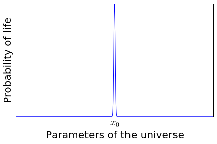
The probability of life is sharply peaked. x0 marks the parameters of the universe that we have in the real world.
Does this graph mean that life is unlikely? No, not necessarily. It depends on the probability distribution of the parameters of the universe. For example, here are three possible probability distributions A, B, and C. Under probability distribution A, or C, life is very unlikely. Under probability distribution B, life is much more likely.
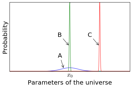
Three possible probability distributions.1
The general idea behind the FTA is that the naturalism hypothesis leads to distribution A, and the God hypothesis leads to distribution B. Since we live in a universe with life (ie at x0), the evidence favors distribution B.
Before we start poking at the probability distributions, I want to comment on the structure of the argument. The tendency among atheists is to think that the FTA is so wrong, that every single step of it must be riddled with problems, down to the very structure of the argument. But in my opinion, the structure is reasonable. Indeed, it is similar to the structure of many arguments in physics.
The tricky question is not “How do we refute the FTA?” The tricky question is “How do we refute the FTA, without also rejecting widely-accepted arguments in physics?” So we’ll start by considering an example from physics.
A digression on inflationary theory
Consider this iconic graph.
Each point on the graph represents observational data. The line that goes through all the different points is the prediction based on the inflationary theory. The gray area above and below the line represents uncertainty, not in the observational data, but uncertainty in the prediction itself. (source)
I’m going to give this digression the attention it deserves, so sit tight. The above graph is considered evidence for inflationary theory, which is the theory that the early universe had a short period of extremely rapid expansion. No, inflationary theory is not the same as Big Bang theory, it’s an auxiliary hypothesis that says the rate of expansion was way way faster than you’d expect, in a very specific way. The rate of expansion was so fast that the effects of quantum fluctuations became writ large in the cosmos, and can be seen as fluctuations in the cosmic microwave background radiation.
Fluctuations come in all sizes. For example, one hemisphere of the sky could be slightly darker than the other hemisphere. Or maybe the sky is divided into quadrants of alternating light and dark. Or maybe the sky is divided into six parts or ten parts or several thousand. The multipole moment (ℓ), shown on the horizontal axis of the graph, is a mathematically precise way of talking about how large a fluctuation we’re talking about. ℓ=1 divides the sky into two parts, and ℓ=1000 divides the sky into much smaller parts.2 There are multiple possible fluctuation “modes” for each value of ℓ; for instance, there are 3 distinct modes with ℓ=1, and 2001 distinct modes with ℓ=1000. So for each value of ℓ, we look at all the modes, and take the average fluctuation strength in those modes.
Inflationary theory does not make precise predictions of the strength of any particular fluctuation mode. Remember, these are quantum fluctuations, they’re fundamentally random. However, inflationary theory makes fairly precise predictions on average fluctuation strengths. And that’s what’s shown in the graph above. The dots show the average strength observed for each value of ℓ. And the line shows the prediction based on inflationary theory. For small values of ℓ, you can see that the predictions are not very precise, because there aren’t enough fluctuations to take a decent average.
Inflationary theory does not predict exactly what the universe looks like. However, it does imply a very specific probability distribution of possible universes. This probability distribution is very sharply peaked, and the peak matches our observations. This is strong evidence for inflationary theory–although it’s not necessarily the last word.
Returning to the FTA
The case of inflation is not unlike the FTA. We start with a theory, we use that theory to predict a probability distribution of outcomes, and show that the probability is sharply peaked, and our observations fit within that peak. There’s nothing unreasonable about this argument structure. Although, you might have noticed a couple differences.
First of all, for inflationary theory we had very precise predictions of the probability distribution, and we can generate further predictions for things we haven’t yet observed.3 In the case of the FTA we basically pulled probability distributions out of our asses. You could say that the probability distribution from the God hypothesis is a bajillion times sharper than the naturalism hypothesis, but if I think there’s a 99% chance that your probability distributions are bullshit, that rather limits the strength of the argument, doesn’t it?
Second of all, if the fluctuations in the cosmic microwave background radiation were different, we could still be around to observe it; whereas if the parameters of the universe were different, then by hypothesis, we would would not be around to see it. It seems that there might be some kind of selection bias at work.
These two differences will be addressed in greater depth in parts 3 and 4, respectively.
1. For the people who like Bayes expressions, the first graph in this post is showing P(L|x), where L is the statement that life exists, and x is the parameters of the universe. The second graph is showing P(x|H), where H is your hypothesis (i.e. either naturalism is true, or God exists). (return)
2. The multipole moment is mathematically identical to concept of angular momentum in atomic orbitals. The s orbital corresponds to ℓ=0, p to ℓ=1, d to ℓ=2, and f to ℓ=3. When I say that ℓ=1 divides the sky into two parts, that’s analogous to how p orbitals have two lobes. But the number of lobes is not completely determined by ℓ. For example, some of the d orbitals have 4 lobes, but one of the d orbitals has only 3 lobes. (return)
3. One observation that we’re all eagerly awaiting is that of the BICEP telescope. They are looking not only at the strength of the cosmic microwave background radiation, but also the polarization. You may recall that BICEP announced proof of inflation in 2015, but that was retracted, and their results are currently inconclusive. (return)
Leave a Reply