Veritasium on the Reproducibility Crisis

It’s a great summary, going into much more depth than most. I really like how Muller brought out a concrete example of publication bias, and found an example of p-hacking in a branch of science that’s usually resistant to it, physics.

But I’m not completely happy with it. Some of this comes from being a Bayesian fanboi that didn’t hear the topic mentioned, but Muller also makes a weird turn of phrase at the end. Muller argues that, as bad as the flaws in science may be, think of how much worse they are in all our other systems of learning about the world.

Slight problem: there are no other systems. Even “I feel it’s true” is based on an evidential claim, evaluated for plausibility against other competing hypotheses. The weighting procedure may be hopelessly skewed, but so too are p-values and the publication process.

Muller could have strengthened his point by bringing up an example, yet did not. We’re left taking his word that science isn’t the sole methodology we have for exploring the world, and that those alternate methodologies aren’t as rigorous. Meanwhile, he explicitly points out that a small fraction of “landmark cancer trials” could be replicated; this implies that cancer treatments, and by extension the well-being of millions of cancer patients, are being harmed by poor methodology in science. Even if you disagree with my assertion that all epistemologies are scientific in some fashion, it’s tough to find a counter-example that effects 40% of us and will kill a quarter.

My hope doesn’t come from a blind assurance that other methodologies are worse than science, it comes from the news that scientists have recognized the flaws in their trade, and are working to correct them. To be fair to Muller, he’d probably agree.

What is False?

John Oliver weighed in on the replication crisis, and I think he did a great job. I’d have liked a bit more on university press departments, who can write misleading press releases that journalists jump on, but he did have to simplify things for a lay audience.

It got me thinking about what “false” means, though. “True” is usually defined as “in line with reality,” so “false” should mean “not in line with reality,” the precise compliment.

But don’t think about it in terms of a single thing, but in multiple data points applied to a specific theory. Suppose we analyze that data, and find that all but a few datapoints are predicted by the hypothesis we’re testing. Does this mean the hypothesis is false, since it isn’t in line with reality in all cases, or true, because it’s more in line with reality than not? Falsification argues that it is false, and exploits that to come up with this epistemology:

  1. Gather data.
  2. Is that data predicted by the hypothesis? If so, repeat step 1.
  3. If not, replace this hypothesis with another that predicts all the data we’ve seen so far, and repeat step 1.

That’s what I had in mind when I said that frequentism works on streams of hypotheses, hopping from one “best” hypothesis to the next. The addition of time changes the original definitions slightly, so that “true” really means “in line with reality in all instances” while “false” means “in at least one instance, it is not in line with reality.”

Notice the asymmetry, though. A hypothesis has to reach a pretty high bar to be considered “true,” and “false” hypotheses range from “in line with reality, with one exception” to “never in line with reality.” Some of those “false” hypotheses are actually quite valuable to us, as John Oliver’s segment demonstrates. He never explains what “statistical significance” means, for instance, but later on uses “significance” in the “effect size” sense. This will mislead most of the audience away from the reality of the situation, and in the absolute it makes his segment “false.” Nonetheless, that segment was a net positive at getting people to understand and care for the replication crisis, so labeling it “false” is a disservice.

We need something fuzzier than the strict binary of falsification. What if we didn’t compliment “true” in the set-theory sense, but in the definitional sense? Let “true” remain “in line with reality in all instances,” but change “false” from “in at least one instance, it is not in reality” to “never in line with reality.” This creates a gap, though: that hypothesis from earlier is neither “true” nor “false,” as it isn’t true in all cases nor false in all. It must be in a third category, as part of some sort of paraconsistent logic.

This is where the Bayesian interpretation of statistics comes from, it deliberately disclaims an absolute “true” or “false” label for descriptions of the world, instead holding them up as two ends of a continuum. Every hypothesis in the third category inbetween, hoping that future data will reveal that its closer to one end of the continuum or the other.

I think it’s a neat way to view the Bayesian/Frequentism debate, as a mere disagreement over what “false” means.

Index Post: P-values

Over the months, I’ve managed to accumulate a LOT of papers discussing p-values and their application. Rather than have them rot on my hard drive, I figured it was time for another index post.

Full disclosure: I’m not in favour of them. But I came to that by reading these papers, and seeing no effective counter-argument. So while this collection is biased against p-values, that’s no more a problem than a bias against the luminiferous aether or humour theory. And don’t worry, I’ll include a few defenders of p-values as well.

What’s a p-value?

It’s frequently used in “null hypothesis significance testing,” or NHST to its friends. A null hypothesis is one you hope to refute, preferably a fairly established one that other people accept as true. That hypothesis will predict a range of observations, some more likely than others. A p-value is simply the odds of some observed event happening, plus the odds of all events more extreme, assuming the null hypothesis is true. You can then plug that value into the following logic:

  1. Event E, or an event more extreme, is unlikely to occur under the null hypothesis.
  2. Event E occurred.
  3. Ergo, the null hypothesis is false.

They seem like a weird thing to get worked up about.

Significance testing is a cornerstone of modern science, and NHST is the most common form of it. A quick check of Google Scholar shows “p-value” shows up 3.8 million times, while its primary competitor, “Bayes Factor,” shows up 250,000. At the same time, it’s poorly understood.

The P value is probably the most ubiquitous and at the same time, misunderstood, misinterpreted, and occasionally miscalculated index in all of biomedical research. In a recent survey of medical residents published in JAMA, 88% expressed fair to complete confidence in interpreting P values, yet only 62% of these could answer an elementary P-value interpretation question correctly. However, it is not just those statistics that testify to the difficulty in interpreting P values. In an exquisite irony, none of the answers offered for the P-value question was correct, as is explained later in this chapter.

Goodman, Steven. “A Dirty Dozen: Twelve P-Value Misconceptions.” In Seminars in Hematology, 45:135–40. Elsevier, 2008. http://www.sciencedirect.com/science/article/pii/S0037196308000620.

The consequence is an abundance of false positives in the scientific literature, leading to many failed replications and wasted resources.

Gotcha. So what do scientists think is wrong with them?

Well, th-

And make it quick, I don’t have a lot of time.

Right right, here’s the top three papers I can recommend:

Null hypothesis significance testing (NHST) is arguably the mosl widely used approach to hypothesis evaluation among behavioral and social scientists. It is also very controversial. A major concern expressed by critics is that such testing is misunderstood by many of those who use it. Several other objections to its use have also been raised. In this article the author reviews and comments on the claimed misunderstandings as well as on other criticisms of the approach, and he notes arguments that have been advanced in support of NHST. Alternatives and supplements to NHST are considered, as are several related recommendations regarding the interpretation of experimental data. The concluding opinion is that NHST is easily misunderstood and misused but that when applied with good judgment it can be an effective aid to the interpretation of experimental data.

Nickerson, Raymond S. “Null Hypothesis Significance Testing: A Review of an Old and Continuing Controversy.” Psychological Methods 5, no. 2 (2000): 241.

After 4 decades of severe criticism, the ritual of null hypothesis significance testing (mechanical dichotomous decisions around a sacred .05 criterion) still persists. This article reviews the problems with this practice, including near universal misinterpretation of p as the probability that H₀ is false, the misinterpretation that its complement is the probability of successful replication, and the mistaken assumption that if one rejects H₀ one thereby affirms the theory that led to the test.

Cohen, Jacob. “The Earth Is Round (p < .05).” American Psychologist 49, no. 12 (1994): 997–1003. doi:10.1037/0003-066X.49.12.997.

This chapter examines eight of the most commonly voiced objections to reform of data analysis practices and shows each of them to be erroneous. The objections are: (a) Without significance tests we would not know whether a finding is real or just due to chance; (b) hypothesis testing would not be possible without significance tests; (c) the problem is not significance tests but failure to develop a tradition of replicating studies; (d) when studies have a large number of relationships, we need significance tests to identify those that are real and not just due to chance; (e) confidence intervals are themselves significance tests; (f) significance testing ensure objectivity in the interpretation of research data; (g) it is the misuse, not the use, of significance testing that is the problem; and (h) it is futile to reform data analysis methods, so why try?

Schmidt, Frank L., and J. E. Hunter. “Eight Common but False Objections to the Discontinuation of Significance Testing in the Analysis of Research Data.” What If There Were No Significance Tests, 1997, 37–64.

OK, I have a bit more time now. What else do you have?

Using a Bayesian significance test for a normal mean, James Berger and Thomas Sellke (1987, pp. 112–113) showed that for p values of .05, .01, and .001, respectively, the posterior probabilities of the null, Pr(H₀ | x), for n = 50 are .52, .22, and .034. For n = 100 the corresponding figures are .60, .27, and .045. Clearly these discrepancies between p and Pr(H₀ | x) are pronounced, and cast serious doubt on the use of p values as reasonable measures of evidence. In fact, Berger and Sellke (1987) demonstrated that data yielding a p value of .05 in testing a normal mean nevertheless resulted in a posterior probability of the null hypothesis of at least .30 for any objective (symmetric priors with equal prior weight given to H₀ and HA ) prior distribution.

Hubbard, R., and R. M. Lindsay. “Why P Values Are Not a Useful Measure of Evidence in Statistical Significance Testing.” Theory & Psychology 18, no. 1 (February 1, 2008): 69–88. doi:10.1177/0959354307086923.

Because p-values dominate statistical analysis in psychology, it is important to ask what p says about replication. The answer to this question is ‘‘Surprisingly little.’’ In one simulation of 25 repetitions of a typical experiment, p varied from .44. Remarkably, the interval—termed a p interval —is this wide however large the sample size. p is so unreliable and gives such dramatically vague information that it is a poor basis for inference.

Cumming, Geoff. “Replication and p Intervals: p Values Predict the Future Only Vaguely, but Confidence Intervals Do Much Better.Perspectives on Psychological Science 3, no. 4 (July 2008): 286–300. doi:10.1111/j.1745-6924.2008.00079.x.

Simulations of repeated t-tests also illustrate the tendency of small samples to exaggerate effects. This can be shown by adding an additional dimension to the presentation of the data. It is clear how small samples are less likely to be sufficiently representative of the two tested populations to genuinely reflect the small but real difference between them. Those samples that are less representative may, by chance, result in a low P value. When a test has low power, a low P value will occur only when the sample drawn is relatively extreme. Drawing such a sample is unlikely, and such extreme values give an exaggerated impression of the difference between the original populations. This phenomenon, known as the ‘winner’s curse’, has been emphasized by others. If statistical power is augmented by taking more observations, the estimate of the difference between the populations becomes closer to, and centered on, the theoretical value of the effect size.

is G., Douglas Curran-Everett, Sarah L. Vowler, and Gordon B. Drummond. “The Fickle P Value Generates Irreproducible Results.” Nature Methods 12, no. 3 (March 2015): 179–85. doi:10.1038/nmeth.3288.

If you use p=0.05 to suggest that you have made a discovery, you will be wrong at least 30% of the time. If, as is often the case, experiments are underpowered, you will be wrong most of the time. This conclusion is demonstrated from several points of view. First, tree diagrams which show the close analogy with the screening test problem. Similar conclusions are drawn by repeated simulations of t-tests. These mimic what is done in real life, which makes the results more persuasive. The simulation method is used also to evaluate the extent to which effect sizes are over-estimated, especially in underpowered experiments. A script is supplied to allow the reader to do simulations themselves, with numbers appropriate for their own work. It is concluded that if you wish to keep your false discovery rate below 5%, you need to use a three-sigma rule, or to insist on p≤0.001. And never use the word ‘significant’.

Colquhoun, David. “An Investigation of the False Discovery Rate and the Misinterpretation of P-Values.” Royal Society Open Science 1, no. 3 (November 1, 2014): 140216. doi:10.1098/rsos.140216.

I was hoping for something more philosophical.

The idea that the P value can play both of these roles is based on a fallacy: that an event can be viewed simultaneously both from a long-run and a short-run perspective. In the long-run perspective, which is error-based and deductive, we group the observed result together with other outcomes that might have occurred in hypothetical repetitions of the experiment. In the “short run” perspective, which is evidential and inductive, we try to evaluate the meaning of the observed result from a single experiment. If we could combine these perspectives, it would mean that inductive ends (drawing scientific conclusions) could be served with purely deductive methods (objective probability calculations).

Goodman, Steven N. “Toward Evidence-Based Medical Statistics. 1: The P Value Fallacy.” Annals of Internal Medicine 130, no. 12 (1999): 995–1004.

Overemphasis on hypothesis testing–and the use of P values to dichotomise significant or non-significant results–has detracted from more useful approaches to interpreting study results, such as estimation and confidence intervals. In medical studies investigators are usually interested in determining the size of difference of a measured outcome between groups, rather than a simple indication of whether or not it is statistically significant. Confidence intervals present a range of values, on the basis of the sample data, in which the population value for such a difference may lie. Some methods of calculating confidence intervals for means and differences between means are given, with similar information for proportions. The paper also gives suggestions for graphical display. Confidence intervals, if appropriate to the type of study, should be used for major findings in both the main text of a paper and its abstract.

Gardner, Martin J., and Douglas G. Altman. “Confidence Intervals rather than P Values: Estimation rather than Hypothesis Testing.” BMJ 292, no. 6522 (1986): 746–50.

What’s this “Neyman-Pearson” thing?

P-values were part of a method proposed by Ronald Fisher, as a means of assessing evidence. Even as the ink was barely dry on it, other people started poking holes in his work. Jerzy Neyman and Egon Pearson took some of Fisher’s ideas and came up with a new method, based on long-term prediction. Their method is superior, IMO, but rather than replacing Fisher’s approach it instead wound up being blended with it, ditching all the advantages to preserve the faults. This citation covers the historical background:

Huberty, Carl J. “Historical Origins of Statistical Testing Practices: The Treatment of Fisher versus Neyman-Pearson Views in Textbooks.” The Journal of Experimental Education 61, no. 4 (1993): 317–33.

While the remainder help describe the differences between the two methods, and possible ways to “fix” their shortcomings.

The distinction between evidence (p’s) and error (a’s) is not trivial. Instead, it reflects the fundamental differences between Fisher’s ideas on significance testing and inductive inference, and Neyman-Pearson’s views on hypothesis testing and inductive behavior. The emphasis of the article is to expose this incompatibility, but we also briefly note a possible reconciliation.

Hubbard, Raymond, and M. J Bayarri. “Confusion Over Measures of Evidence ( p ’S) Versus Errors ( α ’S) in Classical Statistical Testing.” The American Statistician 57, no. 3 (August 2003): 171–78. doi:10.1198/0003130031856.

The basic differences are these: Fisher attached an epistemic interpretation to a significant result, which referred to a particular experiment. Neyman rejected this view as inconsistent and attached a behavioral meaning to a significant result that did not refer to a particular experiment, but to repeated experiments. (Pearson found himself somewhere in between.)

Gigerenzer, Gerd. “The Superego, the Ego, and the Id in Statistical Reasoning.” A Handbook for Data Analysis in the Behavioral Sciences: Methodological Issues, 1993, 311–39.

This article presents a simple example designed to clarify many of the issues in these controversies. Along the way many of the fundamental ideas of testing from all three perspectives are illustrated. The conclusion is that Fisherian testing is not a competitor to Neyman-Pearson (NP) or Bayesian testing because it examines a different problem. As with Berger and Wolpert (1984), I conclude that Bayesian testing is preferable to NP testing as a procedure for deciding between alternative hypotheses.

Christensen, Ronald. “Testing Fisher, Neyman, Pearson, and Bayes.” The American Statistician 59, no. 2 (2005): 121–26.

C’mon, there aren’t any people defending the p-value?

Sure there are. They fall into two camps: “deniers,” a small group that insists there’s nothing wrong with p-values, and the much more common “fixers,” who propose making up for the shortcomings by augmenting NHST. Since a number of fixers have already been cited, I’ll just focus on the deniers here.

On the other hand, the propensity to misuse or misunderstand a tool should not necessarily lead us to prohibit its use. The theory of estimation is also often misunderstood. How many epidemiologists can explain the meaning of their 95% confidence interval? There are other simple concepts susceptible to fuzzy thinking. I once quizzed a class of epidemiology students and discovered that most had only a foggy notion of what is meant by the word “bias.” Should we then abandon all discussion of bias, and dumb down the field to the point where no subtleties need trouble us?

Weinberg, Clarice R. “It’s Time to Rehabilitate the P-Value.” Epidemiology 12, no. 3 (2001): 288–90.

The solution is simple and practiced quietly by many researchers—use P values descriptively, as one of many considerations to assess the meaning and value of epidemiologic research findings. We consider the full range of information provided by P values, from 0 to 1, recognizing that 0.04 and 0.06 are essentially the same, but that 0.20 and 0.80 are not. There are no discontinuities in the evidence at 0.05 or 0.01 or 0.001 and no good reason to dichotomize a continuous measure. We recognize that in the majority of reasonably large observational studies, systematic biases are of greater concern than random error as the leading obstacle to causal interpretation.

Savitz, David A. “Commentary: Reconciling Theory and Practice.” Epidemiology 24, no. 2 (March 2013): 212–14. doi:10.1097/EDE.0b013e318281e856.

The null hypothesis can be true because it is the hypothesis that errors are randomly distributed in data. Moreover, the null hypothesis is never used as a categorical proposition. Statistical significance means only that chance influences can be excluded as an explanation of data; it does not identify the nonchance factor responsible. The experimental conclusion is drawn with the inductive principle underlying the experimental design. A chain of deductive arguments gives rise to the theoretical conclusion via the experimental conclusion. The anomalous relationship between statistical significance and the effect size often used to criticize NHSTP is more apparent than real.

Hunter, John E. “Testing Significance Testing: A Flawed Defense.” Behavioral and Brain Sciences 21, no. 02 (April 1998): 204–204. doi:10.1017/S0140525X98331167.

The Monty Hall Problem, or When the Obvious Isn’t

“You blew it, and you blew it big! Since you seem to have difficulty grasping the basic principle at work here, I’ll explain. After the host reveals a goat, you now have a one-in-two chance of being correct. Whether you change your selection or not, the odds are the same. There is enough mathematical illiteracy in this country, and we don’t need the world’s highest IQ propagating more. Shame!”
– Scott Smith, Ph.D. University of Florida

There was a rather unusual convergence of feminism and skepticism in 1991. Over a thousand people with PhD’s and a few Nobel-prize winners sent angry letters to a puzzle author, insisting the answer to a particular puzzle was wrong. More than a few flashed their academic credentials as evidence in their favor, providing an excellent example of the Argument from Authority. Most seemed to ignore that the author had one of the highest recorded IQs in the world and talked down to her, providing an excellent example of how women’s credentials are frequently undervalued.

The flashpoint for it all was the Monty Hall problem. Here’s how Marilyn vos Savant originally described the problem:

Suppose you’re on a game show, and you’re given the choice of three doors: Behind one door is a car; behind the others, goats. You pick a door, say No. 1, and the host, who knows what’s behind the doors, opens another door, say No. 3, which has a goat. He then says to you, “Do you want to pick door No. 2?” Is it to your advantage to switch your choice?

This wasn’t her invention, but nearly all the people who presented it before were men and I can’t find any evidence they were as heavily doubted. Even a few women shamed vos Savant for coming to the “incorrect” answer, that it’s to your advantage to switch.

On first blush, that does seem incorrect. One door has been removed, leaving two behind and only one with a prize. So there’s a 50/50 chance you picked the right door, right? Even a computer simulation seems to agree.

Out of 12 scenarios, you were better off staying put in 6 of them,
 and switching in 6 of them. So you'll win 50.000000% of the time if you
 stay put, and 50.000000% of the time if you switch.

Out of 887746 trials, you were better off staying put in 444076 of them,
 and switching in 443670 of them. So you'll win 50.022865% of the time if you
 stay put, and 49.977135% of the time if you switch.

But there’s a simple flaw hidden here.

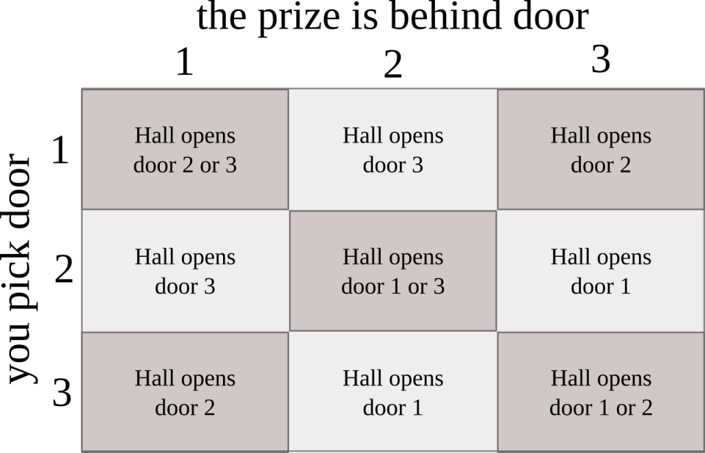
A table of all the outcomes in the Monty Hall problem.You can pick one of three doors, and you have a one in three chance of picking the door with the car. On one of those lucky occasions, Monty Hall opens one of the other doors. Which one doesn’t matter, because it should be obvious that no matter what door he picks your best option is to keep the door you have.

Two-thirds of the time, you’ve picked a door to a goat. Hall can’t open your door yet, and he can’t open the door with the car behind it, so he’s forced to reveal the third door. If you switch, the only sensible choice is the door with the car. If you stay, as already established, you’ve lost.

So two-thirds of the time you should switch, while one-third of the time you’re better off staying put. If you switch all the time, your expected earnings are two-thirds of a car, if you stay put all the time it’s a third of a car, and any strategy that bounces between the two choices (save cheating) will pay off somewhere in between.

In short, always switch.

Still don’t believe me? I’ll modify one of vos Savant’s demonstrations, and show you how to verify this with a deck of cards. Toss out any jokers, then pull out just a single suit of cards and leave the bulk of the deck behind. Grab some way to track the score, while you’re at it, and a coin.

  1. Shuffle the 13 cards well.
  2. Deal out three cards in a horizontal line, face-up. In this game you’re Monty Hall, so there’s no need to hide things.
  3. Find the card with the lowest face value, as that one has the car.
  4. The player always picks the leftmost door.
  5. If they didn’t pick the lowest card, “show” them the other losing door by flipping it over. If they did, toss the coin to determine which of the two losing cards you’ll “show.”
  6. Mark down which strategy wins this round, and gather up the cards.
  7. Repeat from step one until bored or enlightened.

You’ll quickly realize that Hall’s precise choice is irrelevant, and start looping back after step four. After twenty or thirty rounds, you should see the “switch” strategy is superior. If you think I’m cheating by always having the player choose a specific door, you can easily modify the game to be two-player; if you’re suspicious of the thirteen card thing, use three (but shuffle really carefully).

So why did the program give the incorrect answers?

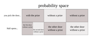
The probability space of the Monty Hall problem; note that not all outcomes are equally likely.While there are four distinct outcomes, they do not carry the same odds of happening. When you pick the door with the car, both choices that Hall can make occupy a third of the probability space in total, whereas both instances where Hall has no choice occupy two-thirds of the space. If you’re not careful, you can give all of them equal weight and falsely conclude that neither strategy has an advantage. If you are careful, you get the proper results.

Out of 9 scenarios, you were better off staying put in 3 of them,
 and switching in 6 of them. So you'll win 33.333332% of the time if you
 stay put, and 66.666664% of the time if you switch.

Out of 2000000 trials, you were better off staying put in 666131 of them,
 and switching in 1333869 of them. So you'll win 33.306549% of the time if you
 stay put, and 66.693451% of the time if you switch.

In hindsight the solution seems obvious enough, but this problem is unusually unintuitive.

Piattelli-Palmarini remarked (see vos Savant, 1997, p. 15): “No other statistical puzzle comes so close to fooling all the people all the time. […] The phenomenon is particularly interesting precisely because of its specificity, its reproducibility, and its immunity to higher education.” He went on to say “even Nobel physicists systematically give the wrong answer, and […] insist on it, and are ready to berate in print those who propose the right answer.” In his book Inevitable illusions: How mistakes of reason rule our minds (1994), Piattelli-Palmarini singled out the Monty Hall problem as the most expressive example of the “cognitive illusions” or “mental tunnels” in which “even the finest and best-trained minds get trapped” (p. 161). [1]

Human beings are only approximately rational; it’s terribly easy to fall for logical fallacies, and act in sexist ways without realizing it. Know thyself, and know how you’ll likely fail.

[1] Krauss, Stefan, and Xiao-Tian Wang. “The psychology of the Monty Hall problem: discovering psychological mechanisms for solving a tenacious brain teaser.Journal of Experimental Psychology: General 132.1 (2003): 3.

A Statistical Analysis of a Sexual Assault Case: Part Three

[complications arise, as does simplicity]

In the last installment, we calculated the odds of nesting or attempted nesting at site 84744 M.S. to be 92%, based on Hugh’s claim. We also found that daufnie_odie’s claim made us 11% confident in nesting.

Hugh, though, was talking about a different point in time. Our original question only asked if the nesting site had seen a nest or attempted nest, without any other clear bounds. It’s similar to asking “will I ever see heads while flipping this coin;” the more distinct observations we have, the greater the chance of at least one head (or nesting attempt) appearing.

The obvious way to combine these two claims is to consider all the possibilities. If we have two independent events, A and B, then the odds of at least one happening is the sum of the first happening but the second not, the second happening but not the first, and both happening. That isn’t too annoying to add up when we have just two events, but if we use this technique for N events we’ll have to consider 2^N – 1 possibilities. Ouch.

Notice, though, that we’re calculating the probability of every possible observation combination, excluding one: that no events occurred. However, by definition the sum of all probabilities must be one. So if we calculate the odds of that single combination and subtract it from one, we know the sum of the odds for every other combination. We can accomplish 2^N – 1 calculations for the cost of one!

Putting this into practice with our numbers above, we calculate the odds of Hugh being wrong about the nest and the odds of daufnie_odie being wrong, then multiply and subtract that from one, and get 93%. A marginal improvement.

But hold on here; why did I multiply those two together? Let’s pull up a diagram:

Dividing the universe by the accounts of Hugh and daufnie_odieOur goal is to figure out A / (A + B + C + D). We can use a bit of algebra to rewrite that as

image

Oh, there’s our multiplication right there! In English, all we have to do is multiply the odds of daufnie_odie being wrong, by the odds of Hugh being wrong when we assume daufne_odie is wrong.

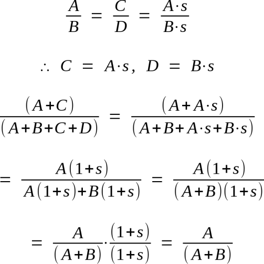
One problem: we don’t know the odds of the latter, just the odds of Hugh being wrong overall. If those two were dependent events, this could be a big problem, but thankfully they’re independent for our purposes; if we’re calculating the odds of no nest or attempt, we don’t care if two or more people are talking about the same event, we just need them to be wrong about whatever they’re talking about. That means that the vertical partition is exactly as it looks in the diagram, a straight cut across the entire probability space. In math terms, the ratio of A to B is the same as that of C to D, which leads to

image

So as long as we can be confident daufnie_odie’s claim is independent of Hugh’s, we can treat (A + B) / (A + B + C + D) as A / (A + B) and just multiply.

But when we take a closer look at daufnie_odie’s post, we realize we’re missing some key facts. They spoke up after reading another post by Pollock Myerson, wondering if the person who contacted them was the same as the one who contacted Myerson. Hopping over to Myerson’s post, we learn that he was introduced to someone claiming to have spotted a nest by Caroline Puppy, and that later on a third person contacted Myerson to validate the original tale. Again no names are mentioned, but Myerson, Puppy, and the third person make it clear that they know this nest claimant.

Scrolling back, we see someone named Bryant Tompsin claiming to know a witness to an attempted nest. This doesn’t look like the same person that contacted Puppy. There’s also a comment by someone who goes by “maryann”, who claims to have spotted at least an attempted nest; whether this is the same person that Tompsin, Puppy or daufnie_odie referred to isn’t clear, but it’s probably not Hugh under a different name.

Scrolling forward, we also find a few posts where Pauline Gray claims to have seen a Sexualis Asoltenti attempt to nest, but leaves out what nesting site she saw it at. Puppy reappears, claiming that she was told by someone named Dijai Gruthi that there was an attempted nesting at 84744 M.S., a fact she later confirmed with someone else who witnessed the same nesting. By comparing photos and accounts, it becomes probable that Pauline Gray was talking about 84744 M.S., that she saw it at the same time as Gruthi, and that Puppy’s other person is Gray. In the meanwhile, Tompsin reappears and also claims to have heard of the same attempted nesting from Gruthi.

As all that’s sinking in, we flip open the local birding magazine and find still more. Pauline Gray admits she really was talking about 84744 M.S. and that Gruthi was present for the attempted nest; the unnamed person of Myerson outs themselves as Ali Smyth, a local birder; and a well-respected person named Jim Grandie suggests he saw a nest or attempt at one but waved it off as horseplay, something birds do when drunk. Biff Jag confirms he was around shortly after Smyth’s nesting observation, and someone with the handle “skippingthem” mentions they know someone who was also a witness. daufnie_odie posts again, and confirms that the nesting Ali Smyth saw was not the one they were aware of. Finally, we can infer some information from the state of the nesting site; if it remains constant, that would suggest a nesting or attempt was unlikely, and if it shifted over time then it likely was nested in at some point. Myerson had a look at the long-term state of 84744 M.S., and indeed found evidence of shifting.

Working through all these combinations would be a nightmare. Fortunately, we don’t have to. As we only care if at least one nest or attempted nest happened, we can instead calculate the odds of no nesting occurring and then subtract that from one. This is a much simpler task, which we’ll accomplish in the next installment

[HJH 2015-07-19: adding some missing links]

A Statistical Analysis of a Sexual Assault Case: Part Two

[the fundamentals of the birds and the bees]

Forget all that talk of sexual assault from last time. Instead, pretend I’m an ornithologist.

Wandering past nesting site 84744 M.S. one day, I wonder if a Sexualis Asoltenti has ever flown in and either nested or attempted to nest there. From various studies, I know the odds of that happening are between six and thirteen percent, making it unlikely. Still, I’m just one person; what have other birdwatchers seen? When I get home, I pull up the favourite web forum for local birders and have a look.

I immediately spot a post by Douglas Hugh, who claims to have seen a nesting Sexualis Asoltenti there. What does that do to the odds? Let’s diagram it out.

The entire universe of possible outcomes.This rectangle represents every possible situation: that no nest exists, that it was made of discarded twine, that Wile E. Coyote instead threw an Acme Portable Hole in there, and so on. We can slice that space by partitioning it into two, one side containing all possibilities where the nest was built or attempted, the other containing the inverse.
Partitioning the probabilities into [I should mention these areas aren’t to scale. I’m just focusing on topology here.]

As this rectangle represents every possibility, it also contains scenarios that include Hugh claiming a nest, as well as Hugh not making any such claim. We can further partition the space.

All possibilities partitioned both by whether or not a nest/attempt was made, and whether or not Hugh claims to have seen a nest.[I should also mention that these boundaries aren’t necessarily accurate. Topology, remember. Also, I wrote this a good three weeks before I saw Jamie’s similar post about Bayes’ Theorem over at SkepChick. Scout’s honour!]

Those previous studies I mentioned represent the area of (A + C) divided by the area of (A + B + C + D).

While we may not know the status of the nest, we do know whether or not Hugh made the claim. Areas C and D are contrary to reality, thus should be dropped from this analysis. The odds of a nest or attempted nest is now the area of A divided by the area of (A + B); in English, that’s the number of instances where Hugh claims a nest, and there is one, as compared to the number of instances where he falsely claims there’s a nest there plus the number of true claims.

As luck would have it, we already have a number to substitute in. Prior research puts the odds of a false nesting claim for Sexualis Asoltenti at between 2-8%; this means that the odds of A / (A + B) are about 92-98%. I’ll take the more conservative value, and say 8% of claims are mistaken, fabricated, or something else. Easy enough.

After figuring all that out, I spot a post from someone named “daufnie_odie.” They claim to have heard a birder mention they’d spotted a nest at 84744 M.S.. No name is given, but the context makes it fairly clear they know this person.

We got lucky last time, because that 8% was for cases where someone claimed they saw a nest or attempted nest, which was exactly the scenario we had. No such luck here, plus there’s a layer of indirection we need to account for. Here’s a first attempt at that:

All probabilities, partitioned by whether there was an attempted/actual nest AND daufnie_odie was approached, vs. daufnie_odie making a claim.On our diagram, the odds of “someone genuinely spots a nest or attempt and mentions it to daufnie_odie” corresponds to the areas where daufnie_odie was approached, A and C, divided by all areas, which is (A + C) / (all). As this box represents all possibilities, and has a total area of one, the odds of the negation of the prior claim (specifically, that there was no nesting, or a false claim, or the news never reaching daufnie_odie), is (1 – (A + C) / (all)) or (B + D) / (all).

Even if that original person saw a nest, though, it’s possible they’d never mention it. We know the first probability, so I’ll put the second at… oh… one third, then multiply the two values together to reach the chance of both events happening.

[Why multiplication? I’ll explicitly cover that in part 3, but if you pay real close attention you’ll get a preview below.]

At this point, I bet a number of you are about to quit in disgust. I just pulled that number out of thin air, and doesn’t that taint the whole enterprise?

If that probability is wildly different from reality, it might. Or, it might not. As I pointed out earlier, if we’re testing the bias of a coin and take a few bad tosses, that could throw off the measurement… but only if we only do a dozen throws. If we do a thousand, it’ll have no significant effect on our final results. Likewise, a bad guess among several good ones will be neutralized, and a lot of fuzzy measurements can combine to create a precise one.

Most importantly, we live in an era of cheap computing. I can run a large number of simulations and check how the parameters change over a wide range of values, giving myself a solid idea of how stable the results are. A little fuzziness is no problem, and who knows? My ad-hoc guess could be bang on the money. This is also handy for anyone who disagrees with my numbers; just plug in your own instead and rerun the analysis.

But back to that. We now need to figure out the odds of daufnie_odie publicly stating their claim, assuming they actually were approached. Maybe they’d forget, or be embarrassed by the situation, but that’s highly unlikely (92%-98% of such claims are legitimate, remember), and this person has some protection by being pseudo-anonymous. I’ll make this probability fairly high, say 95% or so. This corresponds to A / (A + C) in the diagram.

There’s also the possibility that daufnie_odie is making the entire thing up. The pseudo-anonymous argument cuts both ways, also arguing that a false claim is more likely. Nonetheless, an anonymous person that’s careless could be tracked down and held accountable for their words. Given all that, let’s put this probability at an even 50/50. Note that this corresponds to B / (B + D).

Now we can calculate A / (A + B). Multiplying the odds of nesting and this person approaching daufnie_odie, with the odds of daufnie_odie sharing the claim with us, nets us A; multiplying the odds of no nesting or daufnie_odie being approached, with the odds of daufnie_odie making the whole thing up, arrives at B. Put A in the denominator, and the sum of (A + B) in the numerator.

The full math behind daufnie_odie's case. Trust me, it's a bit ugly looking.That’s a pain to write out, though. Let’s clean things up with some substitution; we’ll call the claim “there was a nest or attempted nest and daufnie_odie was approached by a witness” by the letter “H”, and daufnie_odie’s stating that happened will become “E”. To denote the opposite of a claim, like “daufnie_odie did not state he knew of nesting,” we’ll put a little mark in front of it; in this case, that’d look like “¬E”. To refer specifically to the probability of X happening, we’ll say “P(X)”, and if we talk about the odds of X happening given Y did happen, we’ll write “P(X | Y)”. With these simplifications, the math translates into

Bayes' Theorem, in binary mode.Whoops, we’ve accidentally derived a simplified version of Bayes’ Theorem. Ah well, either way we’ve calculated an 11% chance that there was a nest or attempted nest, given daufnie_odie’s post (though as you’ll see later, that number’s a bit naive). As we’re partitioning the probability space, that implies an 89% chance there was no nest or attempt at one.

How do we combine these two accounts together? That’s for part 3

[HJH 2015-06-09: Minor edits for clarity.]
[HJH 2015-06-19: Emphasized daufnie_odie’s probability would change later.]
[HJH 2015-07-19: Adding a missing link.]

A Statistical Analysis of a Sexual Assault Case: Part One

[statistics for the people, and of the people]

I just can’t seem to escape sexual assault. For the span of six months I analysed the Stollznow/Radford case, then finished an examination of Carol Tavris’ talk at TAM2014, so the topic never wandered far from my mind. I’ve bounced my thoughts off other people, sometimes finding support, other times running into confusion or rejection. It’s the latter case that most fascinates me, so I hope you don’t mind if I write my way through the confusion.

The most persistent objection I’ve received goes something like this: I cannot take population statistics and apply them to a specific person. That’s over-generalizing, and I cannot possibly get to a firm conclusion by doing it.

It makes sense on some level. Human beings are wildly different, and can be extremely unpredictable because of that. The field of psychology is scattered with the remains of attempts to bring order to the chaos. However, I’ve had to struggle greatly to reach even that poor level of intellectual empathy, as the argument runs contrary to our every moment of existence. This may be a classic example of talking to fish about water; our unrelenting leaps from the population to the individual seem rare and strange when consciously considered, because these leaps are almost never conscious.

Don’t believe me? Here’s a familiar example.

P1. That object looks like a chair.
P2. Based on prior experience, objects that look like chairs can support my weight.
C1. Therefore, that object can support my weight.

Yep, the Problem of Induction is a classic example of applying the general to the specific. I may have sat on hundreds of chairs in my lifetime, without incident, but that does not prove the next chair I sit on will remain firm. I can even point to instances where a chair did collapse… and yet, if there’s any hesitation when I sit down, it’s because I’m worried about whether something’s stuck to the seat. The worry of the chair collapsing never enters my mind.

Once you’ve had the water pointed out to you, it appears everywhere. Indeed, you cannot do any action without jumping from population to specific.

P1. A brick could spontaneously fly at my head.
P2. Based on prior experience, no brick has ever spontaneously flown at my head.
C1. Therefore, no brick will spontaneously fly at my head.

P1. I’m typing symbols on a page.
P2. Based on prior experience, other people have been able to decode those symbols.
C1. Therefore, other people will decode those symbols.

P1. I want to raise my arm.
P2. Based on prior experience, triggering a specific set of nerve impulses will raise my arm.
C1. Therefore, I trigger those nerve impulses and assume it’ll raise my arm.

“Action” includes the acts of science, too.

P1. I take a measurement with a specific device and a specific calibration.
P2. Based on prior experience, measurements with that device and calibration were reliable.
C1. Therefore, this measurement will be reliable.

Philosophers may view the Problem of Induction as a canyon of infinite width, but it’s a millimetre crack in our day-to-day lives. Not all instances are legitimate, though. Here’s a subtle failure:

P1. This vaccine contains mercury.
P2. Based on prior experience, mercury is a toxic substance with strong neurological effects.
C1. Therefore, this vaccine is a toxic substance with strong neurological effects.

Sure, your past experience may have included horror stories of what happens after chronic exposure to high levels of mercury… but unbeknownst to you, it also included chronic exposure to very low levels of mercury compounds, of varying toxicity, which had no effect on you or anyone else. There’s a stealth premise here: this argument asserts that dosage is irrelevant, something that’s not true but easy to overlook. It’s not hard to come up with similarly flawed examples that are either more subtle (“Therefore, I will not die today”) or less (“Therefore, all black people are dangerous thugs”).

Hmm, maybe this type of argument is unsound when applied to people? Let’s see:

P1. This is a living person.
P2. Based on prior experience, living persons have beating hearts.
C1. Therefore, this living person has a beating heart.

Was that a bit cheap? I’ll try again:

P1. This is a person living in Canada.
P2. Based on prior experience, people living in Canada speak English.
C1. Therefore, this person will speak English.

Now I’m skating onto thin ice. According to StatCan, only 85% of Canadians can speak English, so this is only correct most of the time. Let’s improve on that:

P1. This is a person living in Canada.
P2. Based on prior experience, about 85% of people living in Canada speak English.
C1. Therefore, there’s an 85% chance this person will speak English.

Much better. In fact, it’s much better than anything I’ve presented so far, as it was gathered by professionals in controlled conditions, an immense improvement over my ad-hoc, poorly-recorded personal experience. It also quantifies and puts implicit error bars around what it is arguing. Don’t see how? Consider this version instead:

P1. This is a person living in Canada.
P2. Based on prior experience, about 84.965% of people living in Canada speak English.
C1. Therefore, there’s an 84.965% chance this person will speak English.

The numeric precision sets the implicit error bounds; “about 85%” translates into “from 84.5 to 85.5%.”

Having said all that, it wouldn’t take much effort to track down a remote village in Quebec where few people could talk to me, and the places where I hang out are well above 85% English-speaking. But notice that both are a sub-population of Canada, while the above talks only of Canada as a whole. It’s a solid argument over the domain it covers, but adding more details can change that.

Ready for the next step? It’s a bit scary.

P1. This is a man.
P2. Based on prior experience, between 6 and 62% of men have raped or attempted it.
C1. Therefore, the chance of that man having raped or attempted rape is between 6 and 62%.

Hopefully you can see this is nothing but probability theory at work. The error bars are pretty huge there, but as with the language statistic we can add more details.

P1. This is a male student at a mid-sized, urban commuter university in the United States with a diverse student body.
P2. Based on prior experience, about 6% of such students have raped or attempted it.
C1. Therefore, the odds of that male student having raped or attempted rape is about 6%.

We can do much better, though, by continuing to pile on the evidence we have and watching how the probabilities shift around. Interestingly, we don’t even need to be that precise with our numbers; if there’s sufficient evidence, they’ll converge on an answer. One flip of a coin tells you almost nothing about how fair the process is, while a thousand flips taken together tells you quite a lot (and it isn’t pretty). Even if the numbers don’t come to a solid conclusion, that still might be OK; you wouldn’t do much if there was a 30% chance your ice cream cone started melting before you could lick it, but you would take immediate action if there was a 30% chance of a meteor hitting your house. Fuzzy answers can still justify action, if the consequences are harsh enough and outweigh the cost of getting it wrong.

So why not see what answers we can draw from a sexual assault case? Well, maybe because discussing sexual assault is a great way to get sued, especially when the accused in question is rumoured to be very litigious.

So instead, let’s discuss birds

[HJH 2015-07-19: Changed a link to point to the correct spot.]