Sorry, sorry, got lost in my day job for a bit there. It’s been a month since the fundraising deadline passed, though, and I owe you some follow-up. So, the big question: did we hit the fundraising goal? Let’s load the dataset to find out.
import datetime as dt

import matplotlib.pyplot as pl

import pandas as pd
import pandas.tseries.offsets as pdto


# geez, I really HAVE slacked off
MDT_summer = dt.timezone(offset=dt.timedelta( hours=-6 ))
r1_deadline = dt.datetime( 2020, 6, 12, 23, 59, 59, tzinfo=MDT_summer )


donations = pd.read_csv('donations.cleaned.tsv',sep='\t')

donations['epoch'] = pd.to_datetime(donations['created_at'])

donations['culm'] = donations['amount'].cumsum() + 14723
donations['delta_epoch'] = donations['epoch'] - r1_deadline

donations.tail()| created_at | amount | epoch | culm | delta_epoch | |
|---|---|---|---|---|---|
| 1119 | 2020-06-07T04:56:50-05:00 | 20.0 | 2020-06-07 04:56:50-05:00 | 78499.0 | -6 days +03:56:51 |
| 1120 | 2020-06-07T15:32:00-05:00 | 100.0 | 2020-06-07 15:32:00-05:00 | 78599.0 | -6 days +14:32:01 |
| 1121 | 2020-06-17T16:36:20-05:00 | 50.0 | 2020-06-17 16:36:20-05:00 | 78649.0 | 4 days 15:36:21 |
| 1122 | 2020-06-30T08:53:42-05:00 | 200.0 | 2020-06-30 08:53:42-05:00 | 78849.0 | 17 days 07:53:43 |
| 1123 | 2020-07-01T13:19:00-05:00 | 115.0 | 2020-07-01 13:19:00-05:00 | 78964.0 | 18 days 12:19:01 |
Oof. Nope, instead the fundraiser got stuck at $$78,599, and even the post-deadline donation didn’t get us over the $78,890.69 line. What happened during those sixteen days?
donations['day_epoch'] = donations['delta_epoch'].apply(lambda x: x.days)
mask = (-16 < donations['day_epoch']) & (donations['day_epoch'] < 0)

print( f"There were {sum(mask)} donations over the sixteen day timespan." )
donations[mask]
There were 8 donations over the sixteen day timespan.
| created_at | amount | epoch | culm | delta_epoch | day_epoch | |
|---|---|---|---|---|---|---|
| 1113 | 2020-06-02T08:09:07-05:00 | 100.0 | 2020-06-02 08:09:07-05:00 | 78189.0 | -11 days +07:09:08 | -11 |
| 1114 | 2020-06-02T08:11:25-05:00 | 50.0 | 2020-06-02 08:11:25-05:00 | 78239.0 | -11 days +07:11:26 | -11 |
| 1115 | 2020-06-02T09:54:24-05:00 | 100.0 | 2020-06-02 09:54:24-05:00 | 78339.0 | -11 days +08:54:25 | -11 |
| 1116 | 2020-06-02T13:23:25-05:00 | 20.0 | 2020-06-02 13:23:25-05:00 | 78359.0 | -11 days +12:23:26 | -11 |
| 1117 | 2020-06-02T18:15:55-05:00 | 20.0 | 2020-06-02 18:15:55-05:00 | 78379.0 | -11 days +17:15:56 | -11 |
| 1118 | 2020-06-03T05:45:07-05:00 | 100.0 | 2020-06-03 05:45:07-05:00 | 78479.0 | -10 days +04:45:08 | -10 |
| 1119 | 2020-06-07T04:56:50-05:00 | 20.0 | 2020-06-07 04:56:50-05:00 | 78499.0 | -6 days +03:56:51 | -6 |
| 1120 | 2020-06-07T15:32:00-05:00 | 100.0 | 2020-06-07 15:32:00-05:00 | 78599.0 | -6 days +14:32:01 | -6 |
Looks like the donations came in two bursts, the first about five days after I started the fundraiser, the second on the same day. That in itself is telling, because it tells me that my fundraiser announcement didn't have much effect. What I suspect caused that first burst was not my post, but one by PZ; in other words, either my announcement was too low-profile, I botched it by dragging the thing out over three posts, or I don't have enough readers or interest to trigger many donations.
That insight shapes my plans going forward. For starters, I should stick to two posts per fundraising round, one to kick it off and another a handful of days before deadline to remind everyone of where we're at. I also need to advertise this fundraising drive a bit better, somehow.
I should also mention I've also been mulling the idea of creating a Jupyter notebook or blog post that automatically pulls the latest data from the fundraiser and self-updates; in theory, more feedback should make it easier to see where we're at and encourage more donations. The notebook is easier for me to create, but it can't be hosted on FtB. I had also planned to toss in a donation myself before deadline, as it seems terribly unfair to ask others to open up their wallets without at least a token attempt by myself. That's easy to fix.
print( "   Overall mean/median/mode: ${: 6.2f}/{: 6.2f}/{: 7.2f}".format( \
    donations['amount'].mean(), \
    donations['amount'].median(), \
    donations['amount'].mode().median()) )

print( "Fundraiser mean/median/mode: ${: 6.2f}/{: 6.2f}/{: 7.2f}".format( \
    donations['amount'][mask].mean(), \
    donations['amount'][mask].median(), \
    donations['amount'][mask].mode().median()) )
Overall mean/median/mode: $ 57.15/ 30.00/ 50.00 Fundraiser mean/median/mode: $ 63.75/ 75.00/ 100.00
The central tendencies show some interesting patterns. It looks like the typical donation was higher during the fundraiser period than overall, and there's a skew towards higher-dollar donations. This might seem counter-intuitive, but I think it's a "bullet holes in airplanes" situation: the people struggling most during this pandemic are those with lower or more tentative incomes, and those people are more likely to make smaller donations. When they step back from donating, the average floats up.
The overall category is definitely non-Gaussian, though. Even when there's a skew, the median is always right between the mode and mean. This suggests a multi-modal distribution. Mind if I take a quick detour to check it out?
pl.figure(num=None, figsize=(8, 4), dpi=120, facecolor='w', edgecolor='k')

pl.hist( donations['amount'], bins=20 )

pl.title('Fundraiser Donations')
pl.xlabel('donation amount')
pl.ylabel('frequency')
pl.yscale('log')

pl.show()
That makes more sense. There's a strong skew towards smaller amounts, but a few large donations are tugging the mean upward. If I had to guess, the mode wound up inflated because of psychology; nobody wants to be a $5 donator, so most people will hang on to their funds until they can donate a "non-trivial" amount. $50 seems reasonable, in that regard, as its about the same price as a triple-A game. That's enough to override the Patero distribution you'd expect. The histogram is too granular to verify that guess, though.
pl.figure(num=None, figsize=(8, 4), dpi=120, facecolor='w', edgecolor='k')

pl.hist( donations['amount'], bins=np.linspace(2.5,152.5,155//5) )

pl.title('Fundraiser Donations')
pl.xlim( [0,120] )
pl.xlabel('donation amount')
pl.ylabel('frequency')

pl.show()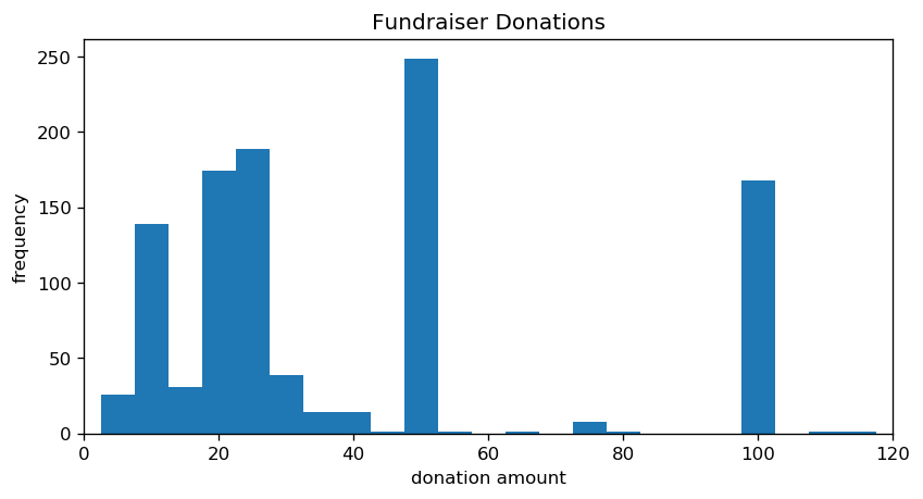
The human love of round numbers really shines through here. There are spikes of $10, $20, $25, $50, and $100 donations, and indeed my guess did pan out. While this was a diversion, this does answer why you'll sometimes hear people explicitly mention small donations: the all-too-human tendency to resist appearing "cheap" is likely causing some people to skip donating when they otherwise can afford to, as the choice in their head is not "how much can I donate?" but instead "can I donate $50?"
Having said that, you've got to watch for overhead. I can't speak for your bank's share, but I know that for Canadians GoFundMe skims off 30 cents per donation plus a fixed percentage. If you donate exactly $5 CAD, then at least 8.9% of that is lost to overhead, whereas donating $50 only loses 3.5% at minimum. The moral: small donations are fine, but bumping up the size of the donation increases its efficiency.
Let's get back on track by calculating the donation rate.
import cmdstanpy as csp

if csp.install_cmdstan():
    print("CmdStan installed.")

x = donations['day_epoch'][mask]
y = donations['culm'][mask]
yerr = donations['amount'].min() * .5     # the minimum donation amount adds some intrinsic uncertainty

lr_model = csp.CmdStanModel(stan_file='linear_regression.stan')
lr_model_fit = lr_model.sample( data = {'N':len(x), 'x':list(x), 'y':list(y), 'y_err':yerr}, \
                              iter_warmup = 10000, iter_sampling = 64 )
print( lr_model_fit.diagnose() )
CmdStan installed. Processing csv files: /tmp/tmp4mjrh6s4/linear_regression-202007092049-1-diixtp68.csv, /tmp/tmp4mjrh6s4/linear_regression-202007092049-2-hlsijp8w.csv, /tmp/tmp4mjrh6s4/linear_regression-202007092049-3-v_zepd83.csv, /tmp/tmp4mjrh6s4/linear_regression-202007092049-4-og66ihyg.csv Checking sampler transitions treedepth. Treedepth satisfactory for all transitions. Checking sampler transitions for divergences. No divergent transitions found. Checking E-BFMI - sampler transitions HMC potential energy. E-BFMI satisfactory for all transitions. Effective sample size satisfactory. The following parameters had split R-hat greater than 1.05: intercept, sigma Such high values indicate incomplete mixing and biasedestimation. You should consider regularizating your model with additional prior information or a more effective parameterization. Processing complete.
This time, we get some error messages, even though I bumped up the number of iterations. That's no surprise, we're only fitting to eight datapoints and so the posterior distribution is much wider and more diffuse. All that effort I put into selecting priors last time is now paying off.
lr_model_names = { v:i for i,v in enumerate(lr_model_fit.column_names) }

flat_chain = list()
for sample in lr_model_fit.sample:
    for chain in sample:
        flat_chain.append( [chain[i] for i in map(lambda x: lr_model_names[x], ['slope', 'intercept', 'sigma'] )] )

print( f"There are {len(flat_chain)} samples in the posterior." )
There are 256 samples in the posterior.
Time to have a look at that posterior.
pl.figure(num=None, figsize=(8, 4), dpi=120, facecolor='w', edgecolor='k')

pl.plot(donations['delta_epoch'].apply(lambda x: x.days),donations['culm'],'-k')
pl_x = np.linspace(-24, 24, 3)
for m,b,_ in flat_chain:
    pl.plot( pl_x, m*pl_x + b, '-r', alpha=0.05 )
pl.title("Defense against Carrier SLAPP Suit, with linear fit")

pl.xlabel("time, days since last donation")
pl.ylabel("fund, dollars")
pl.xlim( [-24, 24] )
pl.ylim( [78000,79000] )
pl.show()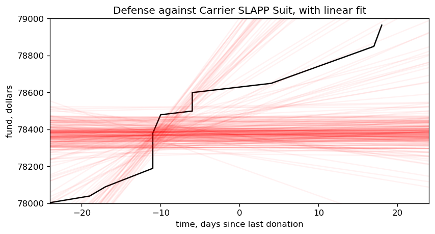
... waaiiitaminute. A lot of those posteriors are flat? And some are negative?!
per_variable = np.array(flat_chain).transpose()

pl.figure(num=None, figsize=(8, 4), dpi=120, facecolor='w', edgecolor='k')

pl.plot( per_variable[0], per_variable[1], '+k')
pl.title("Comparing the slope and intercept values in the posterior")
pl.xlabel("slope")
pl.ylabel("intercept")
pl.show()
Zero is kind of understandable, as it implies no donations have come in, but this is a cumulative graph. It always increases, so negative slopes are impossible! Our model is broken.
We need to fix this, stat. And I think I know how.