I previously explained Bell’s Theorem, which is a “no go” theorem of quantum mechanics. In brief, Bell’s Theorem proved in 1964 that any hidden variable interpretation of quantum mechanics must be nonlocal.
Of course, you may be thinking, maybe the world just is nonlocal, and that hidden information is being passed around faster than light. Unfortunately, there’s another major theorem which makes hidden variable theories even more unpalatable. In 1966-1967, the Kochen-Specker Theorem proved that any hidden variable interpretation must be contextual.
To understand the meaning of “contextual”, suppose we have a quantum cat, and the cat has many possible states. It could be awake or asleep. It could be happy or unhappy. Or the cat could be none of those things because it is dead. Now suppose there are two possible measurements, which answer the following questions:
(1) Is the cat awake, asleep, or dead?
(2) Is the cat happy, unhappy, or dead?
This is a quantum cat, so you can only choose one of the two measurements. However, even if you can’t make both measurements experimentally, you might reasonably expect that the outcomes of the two measurements are related to each other. Specifically, if measurement (1) would find a dead cat, then so would measurement (2), and vice versa. This assumption is called non-contextuality. This cannot be true of hidden variable interpretations of quantum mechanics! Such theories must be contextual.
 Fig. 1: Cat of ambiguous state. Credit: Visentico / Sento
The setup
In discussion of Bell’s theorem, I referred to an electron that could exist in two possible states, spin-up or spin-down. In the language of quantum mechanics, we describe the electron’s state with a two-dimensional vector: (1,0) means spin-up, and (0,1) means spin-down. The cat, however, needs a three dimensional vector: (1,0,0) means awake, (0,1,0) means asleep, and (0,0,1) means dead.
In conventional quantum theory, the cat is not necessarily in one of these three states. For example, the cat might be in state (1,-2,3).1 However, once we measure the cat, it appears in only one of the three states: awake asleep, or dead. The odds ratio of the three outcomes is precisely 1:4:9.2
In a hidden variable theory, we are to imagine that the cat is in exactly one of the three states before we measure it. In other words, the odds ratio is really 1:0:0, 0:1:0, or 0:0:1, and we simply don’t have enough information to determine which one it is.
Now I need to talk about other possible ways to measure the cat. Recall that we could measure electron spin in the vertical direction, or we could measure it in the horizontal direction. In the vector language, spin-right is vector (1,1), while spin-left is (1,-1). In general, we can make a measurement distinguishing between two states only if the vectors corresponding to those states are perpendicular to each other. For example, we can’t measure whether the electron is spin-up or spin-right, since (1,0) is not perpendicular to (1,1). That’s why we can’t measure horizontal and vertical spin simultaneously.
For the cat, we could assign the vector (1,1,0) to the happy state, and (1,-1,0) to the unhappy state. We can make a single measurement distinguishing between three cat states only if those three states are perpendicular to each other. For example, we can distinguish between happy, unhappy, and dead because (1,1,0), (1,-1,0), and (0,0,1) are all perpendicular to each other. I’m going to call three perpendicular states a perpendicular triad (my term).
In summary, each measurement corresponds to a perpendicular triad of vectors. If the cat is described by hidden variables, then the hidden variables must select exactly one of the three vectors to be the outcome of each measurement. The Kochen-Specker theorem shows that this is impossible without contextuality.
Digression: Coloring a plane
As an enthusiast of recreational mathematics, this is where the Kochen-Specker theorem begins to look familiar to me. Consider the following puzzle:
Suppose every point on a plane is colored red or blue. Prove that there exist two points, exactly one unit apart, which are the same color as each other.
Hint: try drawing a triangle. Once you’re done with that one, try the next puzzle:
Suppose every point on a plane is colored red, blue, or green. Prove that there exist two points, exactly one unit apart, which are the same color as each other.
If you give up, search for “Moser Spindle”.
Now, the obvious next question is what happens when you color the plane with four colors? That problem is unsolved! It’s called the Hadwiger-Nelson problem, and it’s part of a notoriously difficult branch of mathematics called Ramsey theory. Ramsey theory also is the source of Graham’s number, allegedly the largest number to ever be seriously used in a proof.
As it turns out, the Kochen-Specker theorem is a Ramsey theory problem. However, instead of coloring a plane, we will attempt to color the surface of a sphere.
The sphere is an abstract representation of the cat’s hidden variables. Each point on the sphere’s surface corresponds to one of the cat’s possible quantum states. Each measurement corresponds to a perpendicular triad of vectors, which corresponds to three points on the sphere, each 90 degrees apart from each other.
 Fig. 2: Cat hiding within sphere. Credit: Meyou Paris.
The coloring of the sphere determines which of the three outcomes will be the one that is measured. Specifically, exactly one of the three points will be red (meaning the cat is in this state), and the other two points will be blue (meaning the cat is not in this state). If the hidden variable theory is non-contextual, then the color of a point depends only on its location on the sphere, and does not depend on your choice of perpendicular triad.
The Kochen-Specker proof
As it turns out, it is impossible to color the sphere while fulfilling the above conditions.
To prove this, we don’t need to consider every single point on the sphere. Rather, we take a finite subset of points on the sphere, and show that there is no satisfactory way to color them. And the number of points required? No more than 33. However, in the original Kochen-Specker proof, there were 117 points. Those points are (un)helpfully illustrated in this pretty graph:
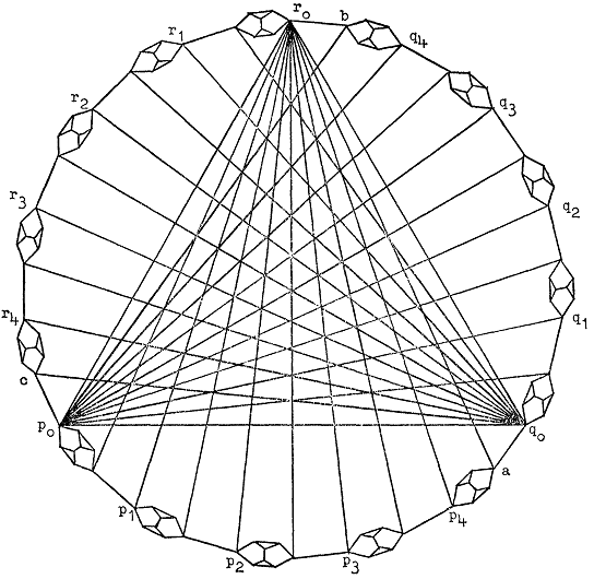
Fig. 3: Kochen Specker theorem in graph form, taken from their paper. Each point corresponds to a point on the sphere. When two points are connected by a line, that means that they are 90 degrees apart from each other (ie “perpendicular”). If you count carefully, there are actually 120 points shown above, but it turns out that three of the points are duplicates.
It looks complicated, but I’ll provide a sketch of the proof for anyone interested. If you aren’t interested, you may skip to the conclusion section.
Here goes. Out of all 117 points, there are 15 points which are particularly important (see Fig. 4). These 15 points appear in a triangle, with the three corners forming a perpendicular triad. Exactly one of these three corners must be colored red. However, according to a lemma we’re about to prove, if a point is colored red, then other points nearby must also be colored red. So starting with a red point in the corner of the triangle, we can hop along the other 15 points, and prove that all of them are red. This is a contradiction, since we said that two of the triangle’s corners must be colored blue.
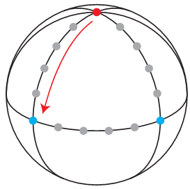 Fig. 4: The backbone of the Kochen Specker proof. The three outermost points form a perpendicular triad.
What remains to be proven is that if a point is colored red, then nearby points must also be colored red. This can be proven using 10 points (see Fig. 5). Here, we assume that point A is red, and seek to prove that point B is red as well.
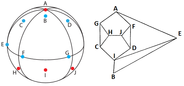 Fig. 5: A proof that nearby points must be the same color. On the left, 10 points are drawn on a sphere (which are not quite to scale). On the right, the relationship between the points is shown using a graph I borrowed from Kochen and Specker. Two points are connected to each other on the graph if they are perpendicular.
The proof is as follows:
(1) First, assume that A is red, and B is blue.
(2) E, F, and G are perpendicular to A, so must be blue.
(3) B, E, and I are a perpendicular triad, so I must be red.
(4) C, and D are perpendicular to I, so must be blue.
(5) C, G, and H are a perpendicular triad, so H must be red.
(6) D, F, and J are a perpendicular triad, so J must be red.
(7) H and J are perpendicular but they are both red. This fails our coloring conditions, so we conclude that (1) was wrong.
This proof is geometrically possible when A and B are sufficiently close to each other–no more than 19.5 degrees apart. This critical angle is calculated in the Kochen-Specker paper, but I won’t calculate it here.
Conclusion
So with all that math, what have we done? We proved that it is impossible to describe the cat’s quantum state with a non-contextual set of hidden variables.
However, as the de Broglie-Bohm interpretation shows, a hidden variable theory of quantum mechanics is nonetheless possible. This is because the de Broglie-Bohm interpretation breaks one of the assumptions we implicitly made, the assumption of contextuality.3 In de Broglie-Bohm theory, what we measure depends on how we measure it.
For many people, this entirely defeats the point of a hidden variable interpretation of quantum theory. The point was to say that an object really is one way or another before we measure it. But there’s no getting around the fact that an object’s properties depend on their measurement.
1. For these quantum states, the length of the vector doesn’t really matter, only the direction. In other words, you could multiply (1,-2,3) by any non-zero factor, even a negative number, and it would still refer to the same quantum state. (return)
2. The odds are calculated by taking the cat’s state, projecting it onto the measured state, and squaring the length of the projection. (return)
3. Similar to Bell’s theorem, physicists have been prodding the Kochen-Specker theorem for decades, and some of have identified other assumptions aside from contextuality–but that’s beyond the scope of this post. (return)
To get an understanding of this which actually makes sense from a Bohmian perspective — since you’re evidently not interested in attempting that in the above, which is fine — I’d recommend the SEC’s entry on Bohmian Mechanics. Assuming a basic understanding of the theory, you may just want to skip to more relevant sections:
10. Quantum Observables
11. Spin
12. Contextuality
(And if there’s still confusion about what it means: 13. Nonlocality)
From (10):
From (12):
Whereas I would say that not having an ontology is not a psychological problem for a physical theory; those need a coherent ontology, or else they are not properly scientific theories about an existing physical world but are about something else. But as a statement about what some think and what price they think they’re paying, as confused as that may be, it seems fair to say that think something like that.
Continuing from (12):
So your example of a live cat, with varying emotional states, or else dead cat, depending on how we “measure” this cat, is not a good analogy to use. Nobody (not a Bohmian at least) is saying that if you measure a cat differently, it will be found to be alive instead of dead — not unless your “measurement” kills the cat, or unless it brings the cat back from the dead, obviously. And you’re not “measuring” what the cat was already like if your “measurement” only tells you that you just killed it or you made it happy or whatever your “measurement” of an “observable” happens to do to the cat.
There are positions in spacetime — those have definite values, definite enough to match experiments, not necessarily an infinitely precise zero-dimensional point where a particle is — and every other “quantum observable” (try actually writing one for a cat, but never mind, we know that you can’t) needs to be understood as deriving from those positions.
Siggy, nicely done.
Lazy folk like me are happy with simpler proofs for higher dimensions, as in the 1996 paper by Cabello et al.
cr @1:
It’s a perfectly good analogy for the purposes of formulating the premises behind the K-S theorem.
You’re contradicting the passage you quoted;
@Rob,
Yeah I saw the 4-dimensional proof first, but I am exceedingly fond of proofs that I can visualize.