I like Dr. R (aka. Dr. Ulrich Schimmack), I’ve relied on his work in the past, but there is one area where we part ways: he’s not a fan of Bayesian statistics.

Like, REALLY not a fan.

It is sad and ironic that Wagenmakers’ efforts to convert psychologists into Bayesian statisticians is similar to Bem’s (2011) attempt to convert psychologists into believers in parapsychology; or at least in parapsychology as a respectable science. While Bem fudged data to show false empirical evidence, Wagenmakers is misrepresenting the way classic statistics works and ignoring the key problem of Bayesian statistics, namely that Bayesian inferences are contingent on prior assumptions that can be gamed to show what a researcher wants to show.  Wagenmaker used this flexibility in Bayesian statistics to suggest that Bem (2011) presented weak evidence for extra-sensory perception.  However, a rebuttle by Bem showed that Bayesian statistics also showed support for extra-sensory perception with different and more reasonable priors.

… Did I cover Bem’s rebuttal? Shoot, I don’t think so. Here’s the quick version: Bem pits an alternative hypothesis fitted to his data against a nil hypothesis; as I found, that strongly favours the existence of precognition. When I instead pitted a more realistic null hypothesis, which allows for some skew due to methodological error or publication bias, against an alternative hypothesis that was based on first principles, the null was triumphant. There’s also some nonsense about “Bayesian” t-tests in there. I should do a proper follow-up, if only to ensure I’m interpreting Bem’s alternative hypothesis correctly.

For now, though, I’m more interested in Dr. R’s discussion of confidence intervals. That means delving into the philosophy behind frequentist statistics.

There’s just one reality that we share, right? This implies that there is one grand theory out there that would explain everything, and a vast number which don’t. Unfortunately, we’re not able to look behind the curtain, so we don’t know that grand theory; we’re stuck inferring what it may be via observation. Worse still, we’re finite creatures with incomplete evidence in front of us, which allows us to be led astray and think we’ve found the grand theory when we haven’t. Our technology can transcend our personal limitations, however, giving us more evidence, more accurate evidence, and pools of conglomerated evidence to analyse.

From all that, frequentism draws the following conclusions: you can’t assign probabilities to hypotheses, because they’re intangible descriptions that can only be true or false; you can’t ever decide a theory is true, though, because that would entail perfect knowledge; but at some point a theory must out itself as false, by diverging from the evidence; and experimental bias can be eliminated by carefully controlling your experimental procedure.

This has a number of consequences, beyond an emphasis on falsification. For one thing, if you’re a frequentist it’s a category error to state the odds of a hypothesis being true, or that some data makes a hypothesis more likely, or even that you’re testing the truth-hood of a hypothesis. For another, if you observe an event that a hypothesis says is rare, you must conclude that the hypothesis should be rejected. There’s also an assumption that you have giant piles of unbiased data at your fingertips, which allows for computational shortcuts: all error follows a Gaussian distribution, maximal likelihoods and averages are useful proxies, the nil hypothesis is valid, and so on.

How does this intersect with confidence intervals? If it’s an invalid move to hypothesise “the population mean is Y,” it must also be invalid to say “there’s a 95% chance the population mean is between X and Z.” That’s attaching a probability to a hypothesis, and therefore a no-no! Instead, what a frequentist confidence interval is really telling you is “assuming this data is a representative sample, if I repeat my experimental procedure an infinite number of times then I’ll calculate a sample mean between X and Z 95% of the time.” A confidence interval says nothing about the test statistic, at least not directly.

Bonkers, right? And yet Dr. R agrees.

… the construction of a confidence interval doesn’t allow us to quantify the probability that an unknown value is within the constructed interval. This probability remains unspecified.

And he gets his interpretation from Jerzy Neyman, no less.

Consider now the case when a sample, S, is already drawn and the calculations have given, say, L = 1 and U = 2. Can we say that in this particular case the probability of the true value of M [the test statistic] falling between 1 and 2 is equal to alpha? The answer is obviously in the negative.

The parameter M is an unknown constant and no probability statement concerning its value may be made, that is except for the hypothetical and trivial ones … which we have decided not to consider.

If you are frequentist, and you’ve ever found yourself saying “there’s a 95% chance the population mean is between X and Z,” or something similar, you are wrong. This is critical, because the article Dr. R is critiquing also attributes this to Neyman:

An X% confidence interval for a parameter θ is an interval (L,U) generated by a procedure that in repeated sampling has an X% probability of containing the true value of θ, for all possible values of θ.

Since that’s not what a true frequentist would ever say, argues Dr. R, and Neyman is about as true a frequentist as you can get, the article is misinterpreting Neyman. He pulls a number of quotes from the original citation to back that up, but somehow neglects to mention these sections:

We may also try to select L(E) and U(E) so that the probability of L(E) falling short of M’ and at the same time of U(E) exceeding M‘, is equal to any number alpha between zero and unity, fixed in advance. If M‘ denotes the true value of M, then of course this probability must be calculated under the assumption that M‘ is the true value of M. […]

The functions L(E) and U(E) satisfying the above conditions will be called the
lower and the upper confidence limits of M. […]

We can then tell the practical statistician that whenever he is certain that the form of the probability law of the X’s is given by the function p ( E | M, N, . . . Z ) which served to determine L(E) and U(E), he may estimate M by making the following three steps : (a) he must perform the random experiment and observe the particular values x1, x2,. . . xn of the X ’s ; (b) he must use these values to calculate the corresponding values of L(E) and U(E) ; and (c) he must state that L(E) < M’ < U(E), where M’ denotes the true value of M.

While Neyman never said that original quote exactly, he did argue for it! This is one of the main reasons why frequentists remain frequentists, they misunderstand their own statistical system, shifting it towards a Bayesian interpretation and thus thinking it has fewer flaws than it does. How else to explain the quality of arguments used to justify frequentism?

Neyman is widely regarded as one of the most influential figures in statistics.  His methods are taught in hundreds of text books, and statistical software programs compute confidence intervals. Major advances in statistics have been new ways to compute confidence intervals for complex statistical problems (e.g., confidence intervals for standardized coefficients in structural equation models; MPLUS; Muthen & Muthen).  What are the a priori chances that generations of statisticians misinterpreted Neyman and committed the fallacy of interpreting confidence intervals after data are obtained?

Given that Neyman held contradictory views of frequentism, also contradicting those of Ronald Fisher and indirectly leading to a Frankenstein’s monster of a statistical system, I reckon they’re pretty good. The Four Temperaments were the most influential methodology in medicine and led to many innovative techniques, yet were comically wrong, so influence says little.

However, if readers need more evidence of psycho-statisticians deceptive practices, it is important to point out that they omitted Neyman’s criticism of their favored approach, namely Bayesian estimation.

Oh no, the authors failed to bring up critiques of Bayesian statistics in an article covering [checks notes] … common misconceptions about confidence intervals. Dr. R also missed the discussion for Figures 4 and 5, which pointed out Bayesian intervals were superior but only if you assumed the Bayesian interpretation of statistics was correct; if you assumed the frequentist interpretation instead, they did second-worst. The authors were fairer than Dr. R paints them.

It is hard to believe that classic statistics are fundamentally flawed and misunderstood because they are used in industry to produce SmartPhones and other technology that requires tight error control in mass production of technology. Nevertheless, this article claims that everybody misunderstood Neyman’s seminal article on confidence intervals.

The abstract states “We show in a number of examples that CIs do not necessarily have any of these properties, and can lead to unjustified or arbitrary inferences. For this reason, we caution against relying upon confidence interval theory to justify interval estimates, and suggest that other theories of interval estimation should be used instead.” Dr. R is exaggerating the claims to make the authors of the article look worse.

And there’s an easy explanation for why frequentism has enjoyed success despite being fundamentally flawed: the extra assumptions it makes above and beyond Bayesian statistics tend to be true, hence why Bayesian and frequentist methods appear to agree so often despite their deep philosophical differences.

So, the problem is not the use of p-values, confidence intervals, or Bayesian statistics.  The problem is abuse of statistical methods.

 

We’re drifting away from a fundamental question, though: if confidence intervals tell you nothing directly about your test statistic, why bother calculating them at all? Dr. R explains:

Nevertheless, we can use the property of the long-run success rate of the method to place confidence in the belief that the unknown parameter is within the interval.  This is common sense. If we place bets in roulette or other random events, we rely on long-run frequencies of winnings to calculate our odds of winning in a specific game.

Hence why I was careful to tack on “directly:” the important part of the confidence interval isn’t the part which falls within it, it’s the part that falls outside. According to frequentism, those values of the test statistic are worthy of rejection. By pooling data, you increase the area outside the interval and narrow down where the truth may lie. You wind up sneaking up on the truth, in the long run.

Let’s put it to the test: I’m going to run a bunch of experiments to determine if the population mean is greater than zero (in reality, it is exactly zero). As usual I’ll assume a Gaussian distribution (correctly, in this case), and calculate confidence intervals as well as use p-values to track statistical significance. Here’s the code, and here’s a graph of the sample means and p-values:

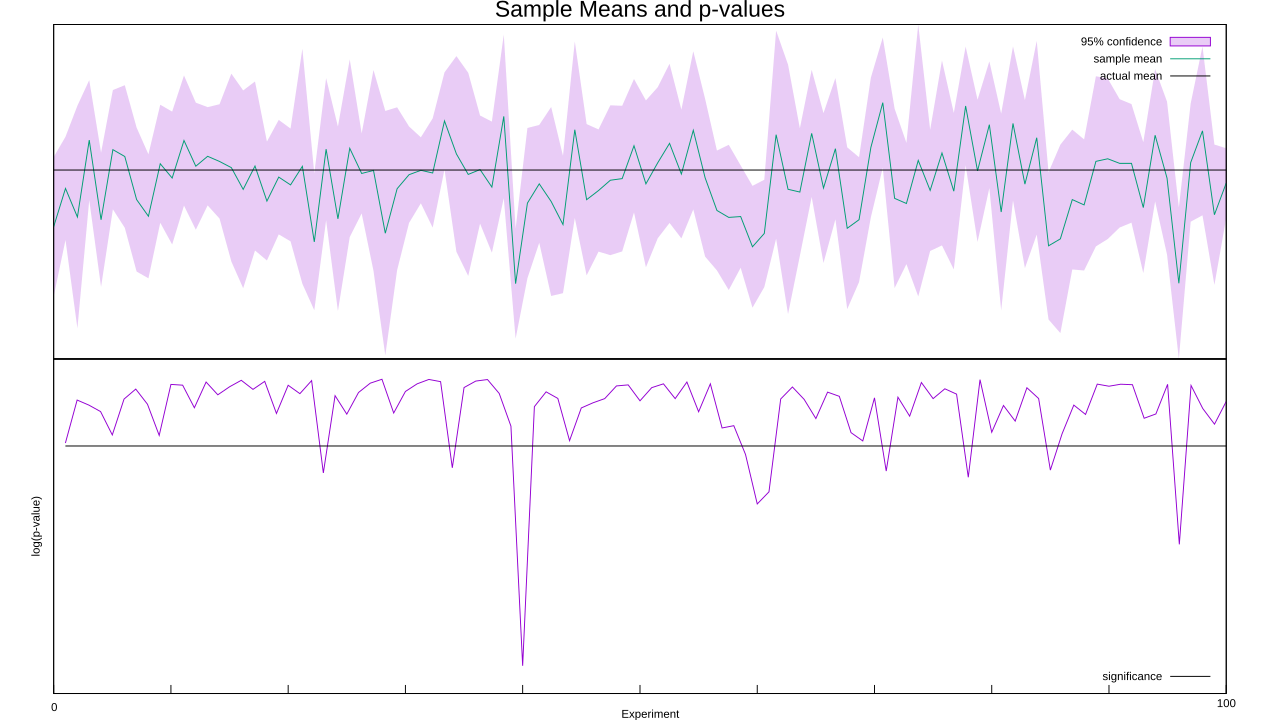
Out of the hundred experiments, ten falsely rejected the null hypothesis. That’s a bit high, as with one-tailed tests and p < 0.05 as our threshold we’d expect only five. Sixty of the experiments had a mean less than zero, too, when we expected fifty. Still, random numbers are random, so fluctuations like these are expected from time to time. So let’s carry on and look at what happens when we pool our data as we go, much as you’d do in a meta-analysis.

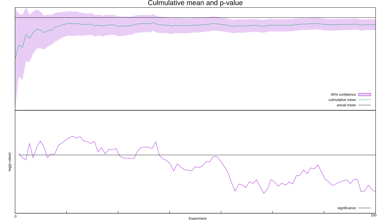
… whaaa?! What the hell went wrong?! Frequentism assumes we’re running an infinite number of tests, but we aren’t. Small fluctuations, such as an excessive number of negative numbers at the start, can throw off a finite number of tests. Your flawless experimental procedure won’t save you here, this problem is baked into the concept of randomness. These early fluctuations can also skew the mean as well as the standard deviation, which in turn mucks up the confidence interval. I deliberately picked the random number seed to create this skew, but if I kept grinding out random numbers the pooled mean will inch closer to zero and the confidence interval will drift back over the zero line. You don’t have to trust me on that one, increase the number of experiments in the above code and see for yourself.

We’re also assuming that we’ve got an unbiased sample, too. That’s not true, thanks to the file-drawer effect: studies that reach statistical significance are a lot more likely to be published than those that don’t. Since any researcher publishing a new effect would be expected to hit statistical significance, this ensures the scientific record starts off skewed, making it tougher for the law of large numbers to hammer flat.

We know the core assumptions of frequentism are false. We know the arguments in favor of it are garbage. So why do we keep using it?

---

[HJH 2018-06-08] Whoops, I just noticed I screwed up my programming code. I assumed I was getting a standard deviation, when I was actually getting the variance! Fortunately the random number generator defaults to a standard deviation of one, and I saw no reason to change it, so the variance and standard deviation are nearly identical. if you compare the old code to the new, you’ll see that the confidence intervals ever-so-sightly tightened up, theoretically making my argument even stronger. Practically, I can’t see a difference between the old and new graphs, so I’m leaving the old ones in place.