The German Tank Problem supposes that there are N tanks with ID numbers from 1 to N. We don’t know what N is, but have looked at a single tank’s ID number, which we’ll denote m. How would you estimate N?
This is a well-known problem in statistics, and you’re welcome to go over to Wikipedia and decide that Wikipedia is a better resource than I am and, you know, fair. But, the particular angle I would like to take, is using this problem to understand the difference between Bayesian and frequentist approaches to statistics.
I’m aware of the popular framing of Bayesian and frequentist approaches as being in an adversarial relationship. I’ve heard some people say they believe that one approach is the correct one and the other doesn’t make any sense. I’m not going to go there. My stance is that even if you’re on Team Bayes or whatever, it’s probably good to understand both approaches at least on a technical level, and that’s what I seek to explain.
In both approaches, we assume that the tank we observe is randomly selected from 1 to N. Therefore, the probability of observing m, conditioned on N is
 = 0")
 = 1/N")
The basic difference is this: The frequentist approach takes this lone assumption and runs with it. The bayesian approach generates stronger answers to the problem, but requires additional assumptions.
The Frequentist approach
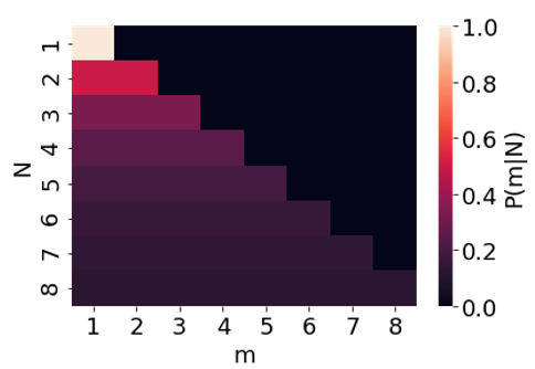
The conditional probability P(m|N) is a function of two variables, m and N. It may be helpful to plot this as a 2D heat map.
We can turn this two-variable function into a single-variable function by holding the other variable constant. This generates two families of functions:
 = P(m|N)")
 = P(m|N)")
Each function p corresponds to a horizontal line in our heat map; for example p4 corresponds to the horizontal line with N = 4. Each function L corresponds to a vertical line in our heat map; for example, L3 corresponds to the vertical line with m = 3.
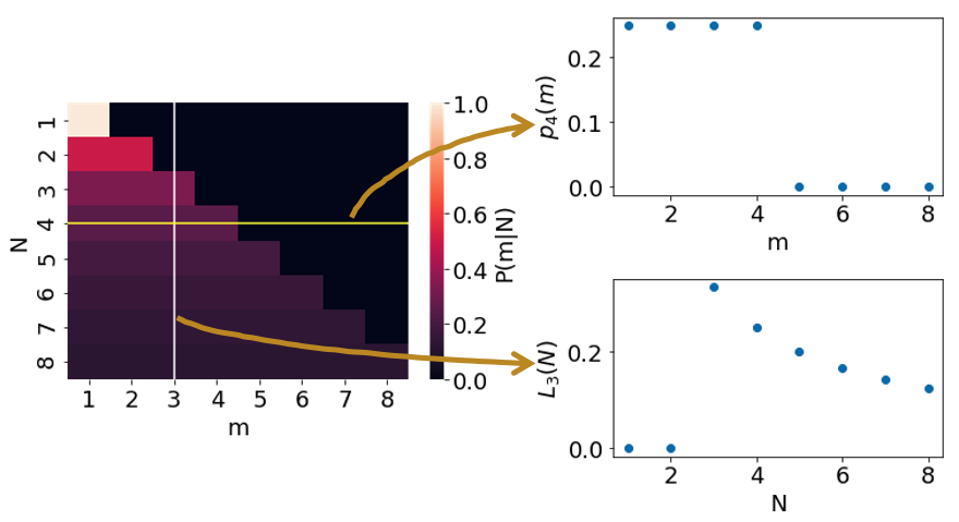
These two families of functions are fundamentally different from each other. pN is a probability distribution function. It has the usual property that the sum of all probabilities is equal to 1. Lm, on the other hand, is what we call a likelihood function. Unlike probabilities, likelihood does not necessarily sum up to 1, and in this case the sum of Lm diverges to infinity.
Now, the ultimate goal of our approach is to “estimate” N, given m. Essentially we want a function f(m) which generates our guess for N. This function is called an estimator. The frequentist framework does not specify which estimator is the “best” one, but I’ll discuss two common types of estimators.
The first is the Maximum Likelihood Estimator, or MLE. This is given by
 = argmax( L_m(N) )")
In the case of the tank problem, MLE(m) = m. So using this estimator, you would guess that the number of tanks is equal to the one ID number you saw.
The second kind of estimator I will discuss is an unbiased estimator. There isn’t necessarily one unique unbiased estimator, “unbiased” is just a property that may apply to multiple estimators, or to none at all. An estimator f(m) is an unbiased estimator of N if
 p_N(m) = N")
for all values of N. Describing this condition in plain language requires a great deal of precision. We start with the assumption of a particular value of N. Then we consider all the possible observations of m, and calculate the value of the estimator for each of those observations. Thus, each value of N implies a probability distribution of the estimator. If the estimator is “unbiased”, then the expected value of the estimator is equal to N.
In the German Tank Problem, there is a single unique unbiased estimator: f(m) = 2m. So if you see the ID number 100, you would guess there are 200 tanks.
The unbiased estimator is fairly reasonable, and is the most-often quoted “answer” to the German Tank Problem. However, the estimator is limited in some ways. For instance, suppose I made you a bet. You pay me a flat amount, and I pay you $N. How much should you be willing to pay me for this bet? You could obey the unbiased estimator, and pay up to $2m. But $2m isn’t the expected payoff of the bet given m, it’s something else entirely, so there’s no guarantee that this strategy is “correct”.
The Bayesian approach
The Bayesian approach is interested in drawing conclusions beyond what is available to the frequentist approach. After all, what is an “unbiased” estimator really? Does it help you win bets? Can you eat it for dinner? And admittedly there’s a communication issue with the frequentist approach, where people confuse likelihood with probability. “Likelihood” is such an arcane concept, and in colloquial language it’s just a synonym for probability. If you’ve ever seen people interpret p-values as probability, that’s precisely the error I’m talking about.
The Bayesian approach seeks a more concrete solution to the problem: The probability distribution of the number of tanks. Once you have this probability distribution, you can estimate the mean number of tanks, the variance, and you can calculate exactly how much money to place in a bet. The catch is that a Bayesian approach requires an additional assumption: the prior probability distribution function, which is to say the probability distribution of the number of tanks before observing any ID numbers.
Using the prior probability distribution P(N), we can use the Bayes theorem to calculate the posterior probability distribution P(N|m).
 = \frac{P(m|N)P(N)}{\sum_k P(m|N=k) P(N=k)}")
Once you have P(N), this formula is rather straightforward to calculate, so I’m skipping that part. Wikipedia has you covered if you want more gory detail. However, Wikipedia, I observe, only solves the problem for a particular choice of P(N). And in my opinion, the wiki obfuscates what its choice of P(N) is. So let’s talk about choosing P(N).
The most common choice of P(N) is a “uniform” distribution. That is, consider every possibility, and assign each possibility an equal prior probability. Or, if N were a continuous variable (i.e. if non-integer number of tanks allowed), then the probability of N being between a and b is proportional to |a-b|.
Unfortunately, “uniform” does not uniquely identify a prior probability distribution. The question is, “uniform in what?” It’s always possible to reframe the question so that the natural uniform distribution looks completely different. For instance, suppose the task were to estimate the number of digits in N. This might lead us to use a distribution that is uniform in the number of digits in N. This leads us to conclude that the probability of N being between 1 and 9 is equal to the probability of N being between 100 and 999. There is no neutral choice of probability distribution.
The German Tank problem has an additional complication, in that a true uniform probability distribution isn’t even possible. There are infinite possible values of N, so if we tried to construct a uniform probability distribution, we would end up with P(N) = 0 everywhere–not a valid probability distribution. One way to deal with this is to place an upper bound on N; for example, allowing N to be uniformly distributed between 1 and Ω. This is the choice that Wikipedia makes, but this leads Wikipedia to the conclusion that the expected number of tanks depends on our choice of Ω. Furthermore, as Ω goes to infinity, the expected number of tanks goes to infinity as well.
Philosophically, P(N) is said to represent your “belief” in N. So the many possible choices of P(N) may reflect the fact that we have different starting beliefs. Generally speaking, Bayesian analysis is most compelling when it a) works for a variety of choices of P(N), or b) P(N) is grounded in some external knowledge, such as an analysis of how many tanks it would be reasonable to produce.
Summary
The German Tank problem is a basic statistics question that can be used to illustrate both the Bayesian and frequentist approaches. The Bayesian approach gives the more concrete solution, in the form of the expected value of the number of tanks. However, the solution depends on additional assumptions, and unfortunately there is no neutral choice of assumptions available. The frequentist approach does not use any additional assumptions, and provides an estimator with a simple form, equal to twice the observed ID number. However, this estimator can be confusing to interpret, and it is technically incorrect to describe it as the expected number of tanks.
Wouldn’t this allow for reasonable estimates as a basis for determining the number? Commercial planes would normally number in the hundreds, military planes in the thousands, tank ten thousands, cars hundreds of thousands, rifles millions. etc.
If you saw a tank with a three digit number, you might expect more. With a six digit number, you might expect it’s near last.
@Intransitive,
Yes exactly. Some external knowledge or intuition is quite valuable for this problem. The Bayes approach is a mathematical formalization of that idea.
I think the best answer is that this is one of those problem where there is not enough information for a meaningful answer. Statistical methods give answers but the upwards margin of error is unlimited and flat, the answer doesn’t really give you any useful information.
@3: Well, if you literally had to make the guess in the dark, you would want one of the options, and there are situations where we actually need to make these kinds of guesses. But it is very true that this is a situation where you have two bad choices and what you’re doing is prioritizing what kinds of risks you care about.
@4 Frederic Bourgault-Christie: If your applying this to a real world problem there is always more information but you also have more problems. The various things Intransitive noted about putting the information in a real world context let you put some sensible limits on the numbers. In the real world you also face the problem that the numbers can be deceptive and the whole situation could be intentional deception. At a simple practical level serial numbers often don’t start at 1. At the deceptive end your enemy could be leaking information about weapon systems that don’t actually exist.
Re “Furthermore, as Ω goes to infinity, the expected number of tanks goes to infinity as well.” I agree that the discussion of the prior part is a bit confusing (at least to me). But “replacing” Ω with infinity in the calculations on the Wiki page do lead to a finite posterior mean, no?
@Christoph Hanck,
Here’s the equation I’m looking at. Under the “one tank” section, the expected number of tanks is given by the last equation:
(Ω-m)/log((Ω-1)/(m-1))
If you take the limit as Ω goes to infinity, this quantity diverges to infinity.
I see – I was referring to the many tanks solution (m-1)(k-1)/(k-2), so that should explain it – thanks!