During the pandemic, I started doing more jigsaw puzzles. Not real puzzles mind you—I found a jigsaw simulator on Steam that was fairly authentic to the real experience. And since I was doing jigsaw puzzles through the medium of video games, I couldn’t help but think about them in the context of puzzle video games. I realized, jigsaw puzzles are kind of weird! In your typical puzzle video game, the ideal is to have a set of levels, each of which require some crucial insight. In contrast, a jigsaw puzzle is more like a large task that you chip away at.
One way of thinking about this is through the lens of computational complexity. Take Sokoban, the classic block pushing puzzle upon which many puzzle video games are founded. In general, a Sokoban puzzle of size N requires exp(N) time to solve, in the worst case. However, the typical Sokoban puzzle does not present the worst case, it presents a curated selection of puzzles that can be solved more quickly. This gives the solver an opportunity to feel clever, rather than just performing a computation.
Jigsaw puzzles, on the other hand, are about performing a computation. And, if you wish to do a large jigsaw puzzle in a reasonable amount of time, you look for ways to perform that computation efficiently. This raises the question: what is the computational complexity of a jigsaw puzzle?
According to the open access paper, “No easy puzzles: Hardness results for jigsaw puzzles” by Michael Brand, realistic jigsaw puzzles require Θ(N2) steps both in the worst case and on average. On the other hand, this is not born out by my own statistics, which seem to fit a straight line.
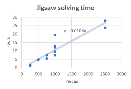
Granted, there’s a major confounding factor. I choose the number of pieces after looking at the image, and generally I’ll choose a larger number of pieces for more detailed images. For science’s sake, I retried the puzzle that took me 24 hours at 2500 pieces, using only 250 pieces, and it took me 50 minutes. That’s about 28 times faster, to do 10 times fewer pieces. Of course, having prior familiarity with the puzzle helps. It’s hard to draw concrete conclusions, but I suspect that my solving time is worse than O(N), but better than O(N2).
In any case, let’s look at the paper to see what’s up.
The paper formulates a jigsaw puzzle in a fairly mathematical way. A puzzle consists of: a set of pieces, a set of positions where pieces could go, and a graph showing which positions are connected to one another. Finally, there are a set of allowable queries that one may ask. For instance, you might ask, “Are pieces X and Y adjacent to each other?”, which is a mathematical representation of trying to fit two pieces together. Another kind of query is “Does piece X go into position Y?” which mathematically represents looking at the picture on the piece and matching it to the picture on the box.
The mathematical object is simplified from a real jigsaw puzzle in a few ways. For instance, it does not concern itself with the orientation of puzzle pieces. And when determining whether pieces are adjacent to one another, it doesn’t distinguish between horizontal or vertical connections or anything like that. But these simplifications are acceptable, because they could only make the mathematical jigsaw easier than a real jigsaw.
My more significant criticism is that this mathematical jigsaw has a more constrained range of queries than a real jigsaw puzzle. In a real jigsaw puzzle, you usually can’t tell exactly where a piece goes in the puzzle, but often you can tell roughly where it goes. You can ask an entirely different kind of query (“Is this piece part of the landscape or part of the sky?”) not accounted for in the mathematical model. The paper states that this does not make a difference to the complexity, but it clearly does.
For instance, in a landscape you can separate land and sky, and further separate land into foreground and background, recursively subdividing categories until you have a bunch of small manageable groups. For a puzzle of size N, we’d need to sort the pieces into O(N) categories, which requires O(logN) per piece. So the computational complexity is O(NlogN).
Another way to illustrate this, is by imagining a puzzle where each piece is labeled with its coordinates. For a puzzle of size N, it takes O(logN) time to read the coordinates of a single puzzle piece. So again, the computational complexity is O(NlogN). The puzzle with coordinates might seem a bit silly, but it’s not that far off from some real puzzles! In a gradient puzzle each piece has a totally unique color, and the color more or less represents its coordinates within the finished puzzle.
(Video shows a gradient puzzle time lapse.)
Of course, I expect the O(NlogN) strategies to eventually break down. It becomes too difficult to subdivide the puzzle into small and readily distinguishable sections. The colors of a gradient puzzle start to become too close together. The coordinates eventually become too long to fit into the pieces with readable font. But “eventually” is irrelevant if we stick to puzzles that are small enough.
This mathematical analysis clarified for me what it means to solve a jigsaw puzzle efficiently, and what sort of techniques may be used to achieve that.
Now, estimate the solving time for that gradient puzzle, assuming the solver had red-green color blindness!
Design and manufacturing technique are relevant I’ve seen puzzles advertised as “most difficult” where
(a) the picture is undifferentiated (e.g. just baked beans, nothing else, or just a sold colour)
(b) there’s little variation in piece design (any piece fits in many places)
(c) the design is printed on both sides, and the puzzle is cut from both sides, so you can’t tell which side is which.