[cn: Bayesian math]
Suppose that I create a test to measure suitability for a particular job. I give this test to a bunch of people, and I find that women on average perform more poorly. Does this mean that women are less suitable for the job, or does it mean that my test is biased against women?
Psychologists do this all the time. They create new tests to measure new things, and then they give the tests to a variety of different groups to observe average differences. So they have a standard statistical procedure to assess whether these tests are biased.
But I recently learned that the standard procedure is mathematically flawed. In fact, rather than producing an unbiased test, the standard procedure practically guarantees a biased test. This is an issue that causes much distress among psychometricians such as Roger Millsap.
Following Millsap, I will describe the standard method for assessing test bias, sketch a proof that it must fail, and discuss some of the consequences.
What is an unbiased test?
Let’s go back to my hypothetical example, where I create a test to measure job suitability. Let’s call the results of this test the JSQ (short for job suitability quotient). It should be clear that JSQ is not the same as job suitability. JSQ is intended to measure job suitability, but there will always be a bit of error. In the language of psychometrics, job suitability is the latent variable, while JSQ is just an indicator.
So let’s suppose that I measure JSQ in men and women, and find that it depends on gender. In mathematical terms, I find that
(1) P( Z | V ) != P( Z ),
where Z is an indicator (JSQ) and V is a demographic variable (gender). What I want to prove is that job suitability depends on gender. In mathematical terms, I want to prove
(2) P( W | V ) != P( W ),
where W is the latent variable (job suitability).
To prove (2), we need to show that the test is unbiased. We say that a test is unbiased if it has measurement invariance. That means it obeys the condition,
(3) P( Z | W, V ) = P( Z | W ).
In English, if two candidates are equally suitable for the job, then the probability distribution of their JSQ scores should be the same regardless of gender. Equations (1) and (3) logically imply (2).
Now, psychologists can’t really measure latent variables. So instead of measurement invariance, they look at a related property called predictive invariance. Basically, they look at how good the test is at predicting outcomes. For example, after measuring JSQ, we might give all the test subjects the job, and then see how well JSQ predicts their later employee evaluations. Predictive invariance means
(4) P( Y | Z, V ) = P( Y | Z ),
where Y is the employee evaluation. In English, two candidates with the same JSQ will have the same probability distribution of employee evaluations, regardless of gender.
Psychologists try to detect testing bias by looking at predictive invariance (4). But the correct definition of test bias is actually measurement invariance (3). So, what is the relationship of measurement invariance and predictive invariance?
Millsap proves that they contradict each other, in the generic case and under basic assumptions. By “generic” I mean that there are some pathological cases where the proof fails, but they aren’t realistic. The “basic assumptions” are Equation (1) and Equation (5) below:
(5) P( Y | W, V ) = P( Y | Z, W, V ).
Equation (5) is called local independence. Basically, Y and Z are both noisy indicators of the latent variable W, and Equation (5) requires that the noise in Y and the noise in Z are uncorrelated to each other.
For reference
In case you forget what anything stands for:
- W is the latent variable. In our example, job suitability.
- Z is an indicator. In our example, the job suitability quotient, or JSQ.
- Y is an indicator, to be predicted by Z. In our example, employee evaluations.
- V is a demographic variable. In our example, gender.
A visual proof
The proof I provide here is not complete, and is not the same as Millsap’s proof. I wanted to come up with something that is visual and accessible, so here it is.
Suppose (in order to prove a contradiction) we have a test where equations (1), (3), (4), and (5) hold true. Also, for simplicity suppose that job suitability, JSQ, and employee evaluations are all continuous variables with the same units (this allows us to plot them together). JSQ and employee evaluations are both indicators of job suitability, but each one introduces some error. We have
(6) JSQ = job suitability + random error
(7) employee evaluation = job suitability + random error
By assumption, the random error in equations (6) and (7) are uncorrelated with each other, and also uncorrelated with gender. So, if we know a person’s job suitability (W=W0), we can predict the distribution of JSQs (Z), and the distribution of employee evaluations (Y). This prediction does not depend on gender.
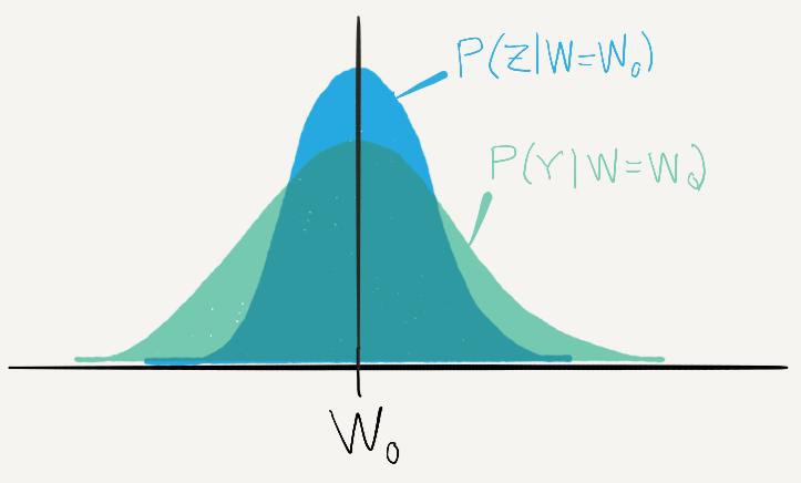
Fig. 1
That’s nice, but that assumes we know a person’s real job suitability. In reality, the only information we might have is their JSQ. Given a particular JSQ (Z=Z0), what is the expected value of their job suitability (W)?
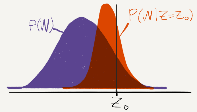
Fig. 2
Here’s the thing. JSQ is an imperfect measure of job suitability, because it introduces random noise. But even if you average over the random noise, JSQ is still an imperfect measure of job suitability. For example, if one person’s JSQ is much higher than average, it’s likely that this is because the random error in the JSQ was in that person’s favor. Therefore, a person with a high JSQ is likely closer to the average than they initially appeared, and will likely get more average employee evaluations later on. This is regression toward the mean.
Now, suppose that the distribution of job suitability is different among men (P1(W)) and women (P2(W)). If this is true, then our prediction of employee evaluations does not just depend on JSQ (Z), but should also depend on gender.
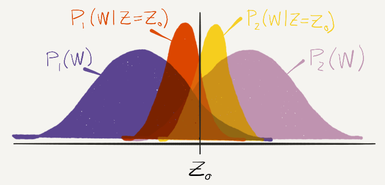
Fig. 3
The conclusion is that a truly unbiased test should violate predictive invariance, which is the thing psychologists use to measure test bias. Rather than proving they have unbiased tests, they are proving the opposite, that they have biased tests.
Concluding remarks
I found this paper troubling to read, because it seems to be saying all of psychology is wrong. But it’s difficult to say just how much of an impact this makes.
One thing the proof does not say, is that psychologists are overestimating group differences. In many cases (including the case I used for the visual proof), psychologists are actually underestimating group differences. In general, the bias can go in either direction.
I also suspect that while predictive invariance and measurement invariance are different, many studies may not have the statistical power to actually detect the difference. If so, then assessing predictive invariance is imperfect, but still the best you can do.
Millsap, for his part, is very concerned that psychologists seem not to have taken notice of his proof. He considers the possibility that psychologists find his work too technical, but dismisses it:
The level of mathematics required to understand the conclusions offered by this work is not high; one does not need to follow the details of the proofs to understand their conclusions.
Having spent a while trying to decipher his papers, I feel that Millsap really didn’t appreciate how hard they are to follow. Reading someone else’s mathematical proof is like reading someone else’s computer programming, only a bunch of steps have been skipped because they’re in a previous publication or because they’re “trivial”. (And I realize that many readers will have difficulty grasping my proof as well. My sympathies to you, I try my best.)
The fact that it’s difficult to understand the proof also makes it difficult to understand the implications. When are psychologists overestimating group differences? When are they underestimating them? And by how much? Readers, I’d love to hear your thoughts.
All of your graphs are normal distributions, what if the distributions aren’t normal?
@colinday,
In my sketch of the proof I used normal distributions, but I believe the proof works for generic distributions.