Ugh, Not Again

P-values are back in the news. Nature published an article, signed by 800 scientists, calling for an end to the concept of “statistical significance.” It ruffled my feathers, even though I agreed with its central thesis.

The trouble is human and cognitive more than it is statistical: bucketing results into ‘statistically significant’ and ‘statistically non-significant’ makes people think that the items assigned in that way are categorically different. The same problems are likely to arise under any proposed statistical alternative that involves dichotomization, whether frequentist, Bayesian or otherwise.

Unfortunately, the false belief that crossing the threshold of statistical significance is enough to show that a result is ‘real’ has led scientists and journal editors to privilege such results, thereby distorting the literature. Statistically significant estimates are biased upwards in magnitude and potentially to a large degree, whereas statistically non-significant estimates are biased downwards in magnitude. Consequently, any discussion that focuses on estimates chosen for their significance will be biased. On top of this, the rigid focus on statistical significance encourages researchers to choose data and methods that yield statistical significance for some desired (or simply publishable) result, or that yield statistical non-significance for an undesired result, such as potential side effects of drugs — thereby invalidating conclusions.

Nothing wrong there. While I’ve mentioned some Bayesian buckets, I tucked away a one-sentence counter-argument in an aside over here. Any artificial significant/non-significant boundary is going to promote the distortions they mention here. What got me writing this post was their recommendations.

What will retiring statistical significance look like? We hope that methods sections and data tabulation will be more detailed and nuanced. Authors will emphasize their estimates and the uncertainty in them — for example, by explicitly discussing the lower and upper limits of their intervals. They will not rely on significance tests. When P values are reported, they will be given with sensible precision (for example, P = 0.021 or P = 0.13) — without adornments such as stars or letters to denote statistical significance and not as binary inequalities (P  < 0.05 or P > 0.05). Decisions to interpret or to publish results will not be based on statistical thresholds. People will spend less time with statistical software, and more time thinking.

This basically amounts to nothing. Journal editors still have to decide what to print, and if there is no strong alternative they’ll switch from an arbitrary cutoff of p < 0.05 to an ad-hoc arbitrary cutoff. In the meantime, they’re leaving flawed statistical procedures in place. P-values exaggerate the strength of the evidence, as I and others have argued. Confidence intervals are not an improvement, either. As I put it:

For one thing, if you’re a frequentist it’s a category error to state the odds of a hypothesis being true, or that some data makes a hypothesis more likely, or even that you’re testing the truth-hood of a hypothesis. […]

How does this intersect with confidence intervals? If it’s an invalid move to hypothesise[sic] “the population mean is Y,” it must also be invalid to say “there’s a 95% chance the population mean is between X and Z.” That’s attaching a probability to a hypothesis, and therefore a no-no! Instead, what a frequentist confidence interval is really telling you is “assuming this data is a representative sample, if I repeat my experimental procedure an infinite number of times then I’ll calculate a sample mean between X and Z 95% of the time.” A confidence interval says nothing about the test statistic, at least not directly.

In frequentism, the parameter is fixed and the data varies. It doesn’t make sense to consider other parameters, that’s a Bayesian move. And yet the authors propose exactly that!

We must learn to embrace uncertainty. One practical way to do so is to rename confidence intervals as ‘compatibility intervals’ and interpret them in a way that avoids overconfidence. Specifically, we recommend that authors describe the practical implications of all values inside the interval, especially the observed effect (or point estimate) and the limits. In doing so, they should remember that all the values between the interval’s limits are reasonably compatible with the data, given the statistical assumptions used to compute the interval. Therefore, singling out one particular value (such as the null value) in the interval as ‘shown’ makes no sense.

Much of what the authors proposed would be fixed by switching to Bayesian statistics. Their own suggestions invoke Bayesian ideas without realizing it. Yet they go out of their way to say nothing’s wrong with p-values or confidence intervals, despite evidence to the contrary. Their proposal is destined to fail, yet it got more support than the arguably-superior p < 0.005 proposal.

Maddening. Maybe it’s time I got out my poison pen and added my two cents to the scientific record.

Gaining Credibility

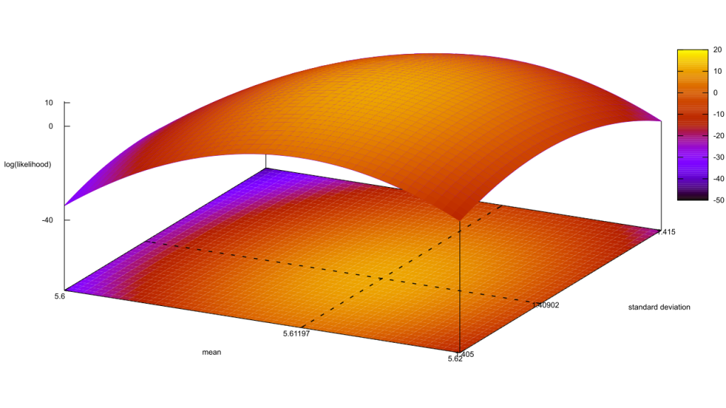
You might have wondered why I didn’t pair my frequentist analysis in this post with a Bayesian one. Two reasons: length, and quite honestly I needed some time to chew over hypotheses. The default frequentist ones are entirely inadequate, for starters:

  • null: The data follows a Gaussian distribution with a mean of zero.
  • alternative: The data follows a Gaussian distribution with a non-zero mean.

In chart form, their relative likelihoods look like this. [Read more…]

Back to Basics

A friend asked for an explainer on Bayesian statistics, and I instinctively reached for Yudkowsky’s only to find this at the top:

This page has now been obsoleted by a vastly improved guide to Bayes’s Theorem, the Arbital Guide to Bayes’s Rule. Please read that instead. Seriously. I mean it.

You can see why once you’ve clicked the link; it asks for your prior experience, then tailors the explanation appropriately. There’s also some good diagrams, and it tries to explain the same concept multiple ways to hammer the point home. Their bit on p-values is on-point, too.

Speaking of stats, I’ve also been drawn back into a course on probability I started years ago. MIT OpenCourseware has a lot of cool offerings, but this entry on probability has been worth my attention. While E.T. Jaynes’ Probability Theory still has my favourite treatment of the subject, the video lectures are easier to parse and proceed at a faster clip.

Abductive and Inferential Science

I love it when Professor Moriarty wanders back to YouTube, and his latest was pretty good. He got into a spot of trouble at the end, which led me to muse on writing a blog post to help him out. I’ve already covered some of that territory, alas, but in the process I also stumbled on something more interesting to blog about. It also effects Sean Carroll’s paper, which Moriarty relied on.

The fulcrum of my topic is the distinction between inference and abduction. The former goes “I have a hypothesis, what does the data say about it?,” while the latter goes “I have data, can I find a hypothesis which explains it?” Moriarty uses this as a refutation of falsification: if we start from the data instead of the hypothesis, we’re not trying to falsify anything! To add salt to the wound, Moriarty argues (and I agree) that a majority of scientific activity consists of abduction and not inference; it’s quite common for scientists to jump from one topic to another, essentially engaging in a tonne of abductive activity until someone forces them to write up a hypothesis. Sean Carroll doesn’t dwell on this as much, but his paper does treat abduction and inference as separate things.

They aren’t separate, at least when it comes to the Bayesian interpretation of statistics. Let’s use a toy example to explain how; here’s a black box with a clear cover:

import ("math/rand")

func blackbox() float64 {

     x := rand.Float64()
     return (4111 + x*(4619 + x*(3627 + x*(7392*x - 9206)))/1213
     }

Each time we turn the crank on this function, we get back a number of some sort. The abductive way to analyse this is pretty straightforward: we grab a tonne of numbers and look for a hypothesis. I’ll go for the mean, median, and standard deviation here, the minimum I’ll need to check for a Gaussian distribution.

Samples = 1000001
Mean    = 5.61148
Std.Dev = 1.40887
Median  = 5.47287

Looks like there’s a slight skew downwards, but it’s not that bad. So I’ll propose that the output of this black box follows a Gaussian distribution, with mean 5.612 and standard deviation 1.409, until I can think of a better hypothesis which handles the skew.

After we reset for the inferential analysis, we immediately run into a problem: this is a black box. We know it has no input, and outputs a floating-point number, and that’s it. How can we form any hypothesis, let alone a null and alternative? We’ve no choice but to make something up. I’ll set my null to be “the black box outputs a random floating-point number,” and the alternative to “the output follows a Gaussian distribution with a mean of 0 and a standard deviation of 1.” Turn the crank, aaaand…

Samples            = 1000001
log(Bayes Factor)  = 26705438.01142
  (That means the most likely hypothesis is H1 (Gaussian distribution, mean = 0, std.dev = 1))

Unsurprisingly, our alternative does a lot better than our null. But our alternative is wrong! We’d get that impression pretty quickly if we watched the numbers streaming in. There’s an incredible temptation to take that data to refine or propose a new hypothesis, but that’s an abductive move. Inference is really letting us down.

Worse, this black box isn’t too far off from the typical science experiment. It’s rare any researcher is querying a black box, true, but it’s overwhelmingly true that they’re generating new data without incorporating other people’s datasets. It’s also rare you’re replicating someone else’s work; most likely, you’re taking existing ideas and rearranging them into something new, so prior findings may not carry forward. Inferential analysis is more tractable than I painted it, I’ll confess, but the limited information and focus on novelty still favors the abductive approach.

But think a bit about what I did on the inferential side: I picked two hypotheses and pitted them against one another. Do I have to limit myself to two? Certainly not! Let’s rerun the analysis with twenty-two hypotheses: the flat distribution we used as a null before, plus twenty-one alternative hypotheses covering every integral mean from -10 to 10 (though keeping the standard deviation at 1).

Samples                                 = 100001
log(likelihood*prior), H0               = -4436161.89971
log(likelihood*prior), H1, mean = -10   = -12378220.82173
log(likelihood*prior), H1, mean =  -9   = -10866965.39358
log(likelihood*prior), H1, mean =  -8   = -9455710.96544
log(likelihood*prior), H1, mean =  -7   = -8144457.53730
log(likelihood*prior), H1, mean =  -6   = -6933205.10915
log(likelihood*prior), H1, mean =  -5   = -5821953.68101
log(likelihood*prior), H1, mean =  -4   = -4810703.25287
log(likelihood*prior), H1, mean =  -3   = -3899453.82472
log(likelihood*prior), H1, mean =  -2   = -3088205.39658
log(likelihood*prior), H1, mean =  -1   = -2376957.96844
log(likelihood*prior), H1, mean =   0   = -1765711.54029
log(likelihood*prior), H1, mean =   1   = -1254466.11215
log(likelihood*prior), H1, mean =   2   = -843221.68401
log(likelihood*prior), H1, mean =   3   = -531978.25586
log(likelihood*prior), H1, mean =   4   = -320735.82772
log(likelihood*prior), H1, mean =   5   = -209494.39958
log(likelihood*prior), H1, mean =   6   = -198253.97143
log(likelihood*prior), H1, mean =   7   = -287014.54329
log(likelihood*prior), H1, mean =   8   = -475776.11515
log(likelihood*prior), H1, mean =   9   = -764538.68700
log(likelihood*prior), H1, mean =  10   = -1153302.25886
  (That means the most likely hypothesis is H1 (Gaussian distribution, mean = 6, std.dev = 1))

Aha, the inferential approach has finally gotten us somewhere! It’s still wrong, but you can see the obvious solution: come up with as many hypotheses as you can to explain the data, before we look at it, and run them all as the data rolls in. If you’re worried about being swamped by hypotheses, I’ve got a word for you: marginalization. Bayesian statistics handles hypotheses with parameters by integrating over all of them; you can think of these as composites, a mash of point hypotheses which collectively do a helluva lot better at prediction than any one hypothesis in isolation. In practice, then, Bayesians have always dealt with large numbers of hypotheses simultaneously.

The classic example of this is conjugate priors, where we carefully combine hyperparameters to evaluate a potentially infinite family of probability distributions. In fact, let’s try it right now: the proper conjugate here is the Normal-Inverse-Gamma, as we’re tracking both the mean and standard deviation of Gaussian distributions.

Samples = 1000001
μ       = 5.61148
λ       = 1000001.00000
α       = 500000.50000
β       = 992457.82655

median  = 5.47287

That’s a good start, μ lines up with the mean we calculated earlier, and λ is obviously the sample count. The shape of the posteriors is still pretty opaque, though; we’ll need to chart this out by evaluating the Normal-Inverse-Gamma PDF a few times.Conjugate posterior for the collection of all Gaussian distributions which could describe the data.Excellent, the inferential method has caught up to abduction! In fact, as of now they’re both working identically. Think: what’s the difference between a hypothesis you proposed before collecting the data, and one you proposed after? In frequentism, the stopping problem implies that we could exit early and falsely reject our null, when data coming down the pipe would have pushed it back to “fail to reject.” There, the choice of hypothesis could have an influence on the outcome, so there is a difference between the two cases. This is made worse by frequentism’s obsession over one hypothesis above all others, the null.

Bayesian statistics is free of that problem, because every hypothesis is judged on their relative likelihood in reference to a dataset shared by all hypotheses. There is no stopping problem baked into the methodology. Whether I evaluate any given hypothesis before or after I collect the data is irrelevant, because either way it has to cope with all the data. This also frees me up to invent hypotheses whenever I wish.

But this also defeats the main attack against falsification. The whole point of invoking abduction was to save us from asserting any hypotheses in the beginning; if there’s no difference in when we invoke our hypotheses, however, then falsification might still apply.

Here’s where I return to giving Professor Moriarity a hand. He began that video by saying scientists usually don’t engage in falsification, hence it cannot be The Scientific Method, but ended it by approvingly quoting Feynman: “We are trying to prove ourselves wrong as quickly as possible, because only in that way can we find progress.” Isn’t that falsification, right there?

This is yet another area where frequentist and Bayesian statistics diverge. As I pointed out earlier, frequentism is obsessed with falsifying the null hypothesis and trying to prove it wrong. Compare and contrast with what past-me wrote about Bayes Factors:

If data comes up that doesn’t square well with a hypothesis, its certainty takes a hit. But if we’re comparing it to another hypothesis that also doesn’t predict the data, the Bayes Factor will remain close to 1 and our certainties won’t shift much at all. Likewise, if both hypotheses strongly predict the data, the Factor again stays close to 1. If we’re looking to really shift our certainty around, we need a big Bayes Factor, which means we need to find scenarios where one hypothesis strongly predicts the data while the other strongly predicts this data shouldn’t happen.

Or, in other words, we should look for situations where one theory is… false. That sounds an awful lot like falsification!

But it’s not the same thing. Scroll back up to that Normal-Inverse-Gamma PDF, and pick a random point on the graph. The likelihood at that point is less than the likelihood at the maximum point. If you were watching those two points as we updated with new data, your choice would have gradually gone from about equally likely to substantially less likely. Your choice is more likely to be false, all things being equal, but it’s also not false with a capital F. Maybe the first million data points were a fluke, and if we continued sampling to a billion your choice would roar back to the top? This is the flip-side of having no stopping problem: the door is always left open a crack for any crackpot hypotheses to make a comeback.

Now look closely at the scale of the vertical axis. That maximal likelihood is well above 100%! In fact it’s somewhere around 4,023,000% by my calculations. While the vast majority are dropping downwards, there’s an ever-shrinking huddle of points that are becoming more likely as data is added! Falsification should only make things less likely, however.

Under Bayesian statistics, falsification is treated as a heuristic rather than a core part of the process. We’re best served by trying to find areas where hypotheses differ, yet we never declare one hypothesis to be false. This saves Moriarty: he’s both correct in disclaiming falsification, and endorsing the process of trying to prove yourself wrong. The confusion between the two stems from having to deal with two separate paradigms that appear to have substantial overlap, even though a closer look reveals fundamental differences.

Feeling the Research

Daryl Bem must be sick of those puns by now.

Back in 2011 he published Feeling the Future, a paper that combined multiple experiments on human precognition to argue it was a thing. Naturally this led to a flurry of replications, many of which riffed on his original title. I got interested via a series of blog posts I wrote that, rather surprisingly, used what he published to conclude precognition doesn’t exist.

I haven’t been Bem’s only critic, and one that’s a lot higher profile than I has extensively engaged with him both publicly and privately. In the process, they published Bem’s raw data. For months, I’ve wanted to revisit that series with this new bit of data, but I’m realising as I type this that it shouldn’t live in that Bayes 20x series. I don’t need to introduce any new statistical tools to do this analysis, for starters; all the new content here relates to the dataset itself. To make understanding that easier, I’ve taken the original Excel files and tossed them into a Google spreadsheet. I’ve re-organized the sheets in order of when the experiment was done, added some new columns for numeric analysis, and popped a few annotations in.

Odd Data

The first thing I noticed was that the experiments were not presented in the order they were actually conducted. It looks like he re-organized the studies to make a better narrative for the paper, implying he had a grand plan when in fact he was switching between experimental designs. This doesn’t affect the science, though, and while never stating the exact order Bem hints at this reordering on pages three and nine of Feeling the Future.

What may affect the science are the odd timings present within many of the datasets. As Dr. R pointed out in an earlier link, Bem combined two 50-sample studies together for the fifth experiment in his paper, and three studies of 91, 19, and 40 students for the sixth. Pasting together studies like that is a problem within frequentist statistics, due to the “stopping problem.” Stopping early is bad, because random fluctuations may blow the p-value across the “statistically significant” line when additional data would have revealed a non-significant result; but stopping too late is also bad, because p-values tend to exaggerate the evidence against the null hypothesis and the problem gets worse the more data you add.

But when pouring over the datasets, I noticed additional gaps and oddities that Dr. R missed. Each dataset has a timestamp for when subjects took the test, presumably generated by the hardware or software. These subjects were undergrad students at a college, and grad students likely administered some or all the tests. So we’d expect subject timestamps to be largely Monday to Friday affairs in a continuous block. Since these are machine generated or copy-pasted from machine-generated logs, we should see a monotonous increase.

Yet that 91 study which makes up part of the sixth study has a three-month gap after subject #50. Presumably the summer break prevented Bem from finding subjects, but what sort of study runs for a month, stops for three, then carries on for one more? On the other hand, that logic rules out all forms of replication. If the experimental parameters and procedure did not change over that time-span, either by the researcher’s hand or due to external events, there’s no reason to think the later subjects differ from the former.

Look more carefully and you see that up until subject #49 there were several subjects per day, followed by a near two-week pause until subject #50 arrived. It looks an awful like Bem was aiming for fifty subjects during that time, was content when he reached fourty-nine, then luck and/or a desire for even numbers made him add number fifty. If Bem was really aiming for at least 100 subjects, as he claimed in a footnote on page three of his paper, he could have easily added more than fifty, paused the study, and resumed in the fall semester. Most likely, he was aiming for a study of fifty subjects back then, suggesting the remaining forty-one were originally the start of a second study before later being merged.

Experiment 1, 2, 4, and 7 also show odd timestamps. Many of these can be explained by Spring Break or Thanksgiving holidays, but many also stop at round numbers. There’s also instances where some timestamps occur out-of-order or the sequence number reverses itself. This is pretty strong evidence of human tampering, though “tampering” isn’t the synonymous with “fraud;” any sufficiently large study will have mistakes, and any attempt to correct those mistakes will look like fraud. That still creates uncertainty in a dataset and necessarily lowers our trust in it.

I’ve also added stats for the individual runs, and some of them paint an interesting tale. Take experiment 2, for instance. As of the pause after subject #20, the success rate was 52.36%, but between subject #20 and #100 it was instead 51.04%. The remaining 50 subjects had a success rate of 52.39%, bringing the total rate up to 51.67%. Why did I place a division between those first hundred and last fifty? There’s no time-stamp gap there, and no sign of a parameter shift. Nonetheless, if we look at page five and six of the paper, we find:

For the first 100 sessions, the flashed positive and negative pictures were independently selected and sequenced randomly. For the subsequent 50 sessions, the negative pictures were put into a fixed sequence, ranging from those that had been successfully avoided most frequently during the first 100 sessions to those that had been avoided least frequently. If the participant selected the target, the positive picture was flashed subliminally as before, but the unexposed negative picture was retained for the next trial; if the participant selected the nontarget, the negative picture was flashed and the next positive and negative pictures in the queue were used for the next trial. In other words, no picture was exposed more than once, but a successfully avoided negative picture was retained over trials until it was eventually invoked by the participant and exposed subliminally. The working hypothesis behind this variation in the study was that the psi effect might be stronger if the most successfully avoided negative stimuli were used repeatedly until they were eventually invoked.

So precisely when Bem hit a round number and found the signal strength was getting weaker, he tweaked the parameters of the experiment? That’s sketchy, especially if he peeked at the data during the pause at subject #20. If he didn’t, the parameter tweak is easier to justify, as he’d already hit his goal of 100 subjects and had time left in the semester to experiment. Combining both experimental runs would still be a no-no, though.

Uncontrolled Controls

Bem’s inconsistent use of controls was present in the paper, but it’s a lot more obvious in the dataset. In experiments 2, 3, 4, and 7 there is no control group at all. That is dangerous. If you run a control group through a protocol nearly identical to that of the experimental group, and you don’t get a null result, you’ve got good evidence that the procedure is flawed. If you don’t run a control group, you’d better be damn sure your experimental procedure has been proven reliable in prior studies, and that you’re following the procedure close enough to prevent bias.

Bem doesn’t hit that for experiments 2 and 7; the latter isn’t the replication of a prior study he’s carried out, and while the former is a replication of experiment 1 the earlier study was carried out two years before and appears to have been two separate sample runs pasted together, each with different parameters. In experiments 3 and 4, Bem’s comparing something he knows will have an effect (forward priming) with something he hopes will have an effect (retroactive priming). There’s no explicit comparison of the known-effect’s size to that found in other studies, Bem’s write-up appears to settle for showing statistical significance. Merely showing there is an effect does not demonstrate that effect is of the same magnitude as expected.

Conversely, experiments 5 and 6 have a very large number of controls, relative to the experimental conditions. This is wasteful, certainly, but it could also throw off the analysis: since the confidence interval narrows as more samples are taken, we can tighten one side up by throwing more datapoints in and taking advantage of the p-value’s weakness.

Experiment 6 might show this in action. For the first fifty subjects, the control group was further from the null value than the negative image group, but not as extreme as the erotic image one. Three months later, the next fourty-one subjects are further from the null value than both the experimental groups, but this time in the opposite direction! Here, Bem drops the size of the experimental groups and increases the size of the control group; for the next nineteen subjects, the control group is again more extreme than the negative image group and again less extreme than the erotic group, plus the polarity has flipped again. For the last fourty subjects, Bem increased the sizes of all groups by 25%, but the control is again more extreme and the polarity has flipped yet once more. Nonetheless, adding all four runs together allows all that flopping to cancel out, and Bem to honestly write “On the neutral control trials, participants scored at chance level: 49.3%, t(149) = -0.66, p = .51, two-tailed.” This looks a lot like tweaking parameters on-the-fly to get a desired outcome.

It also shows there’s substantial noise in Bem’s instruments. What’s the odds that the negative image group success rate would show less variance than the control group, despite having anywhere from a third to a sixth of the sample size? How can their success rate show less variance than the erotic image group, despite having the same sample size? These scenarios aren’t impossible, but with them coming at a time when Bem was focused on precognition via negative images it’s all quite suspicious.

The Control Isn’t a Control

All too often, researchers using frequentist statistics get blinded by the way p-values ignore the null hypothesis, and don’t bother checking their control groups. Bem’s fairly good about this, but we can do better.

All of Bem’s experiments, save 3 and 4, rely on Bernoulli processes; every person has some probability of guessing the next binary choice correctly, due possibly to inherent precognitive ability, and that probability does not change with time. It follows that the distribution of successful guesses follows the binomial distribution, which can be written:

P( s `divides` p,f ) ~=~ { (s+f)"!" } over { s"!" f"!" } p^s ( 1-p )^f where s is the number of successes, f the number of failures, and p the odds of success; that means P ( s | p,f ) translates to “the probability of having s successes, given the odds of success are p and there were f failures.” Naturally, p must be between 0 and 1.

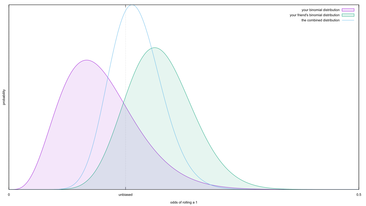
Let’s try a thought experiment: say you want to test if a single six-sided die is biased to come up 1. You roll it thirty-six times, and observe four instances where it comes up 1. Your friend tosses it seventy-two times, and spots fifteen instances of 1. You’d really like to pool your results together and get a better idea of how fair the die is; how would you do this? If you answered “just add all the successes together, as well as the failures,” you nailed it!The probability distribution of rolling a 1 for a given die, according to you and your friend's experiments.The results look pretty good; both you and your friend would have suspected the die was biased based on your individual rolls, but the combined distribution looks like what you’d expect from a fair die.

But my Bayes 208 post was on conjugate distributions, which defang a lot of the mathematical complexity that comes from Bayesian methods by allowing you to merge statistical distributions. Sit back and think about what just happened: both you and your friend examined the same Bernoulli process, resulting in two experiments and two different binomial distributions. When we combined both experiments, we got back another binomial distribution. The only way this differs from Bayesian conjugate distributions is the labeling; had I declared your binomial to be the prior, and your friend’s to be the likelihood, it’d be obvious the combination was the posterior distribution for the odds of rolling a 1.

Well, almost the only difference. Most sources don’t list the binomial distribution as the conjugate for this situation, but instead the Beta distribution:

Beta( p `divides` %alpha,%beta ) ~=~ { %GAMMA(%alpha + %beta) } over { %GAMMA(%alpha) %GAMMA(%beta) } p^{%alpha-1} ( 1-p )^{%beta-1}

But I think you can work out the two are almost identical, without any help from me. The only real advantage of the Beta distribution is that it allows non-integer successes and failures, thanks to the Gamma function, which in turn permits a nice selection of priors.

In theory, then, it’s dirt easy to do a Bayesian analysis of Bem’s handiwork: tally up the successes and failures from each individual experiment, add them together, and plunk them into a binomial distribution. In practice, there are three hurdles. The easy one is the choice of prior; fortunately, Bem’s datasets are large enough that they swamp any reasonable prior, so I’ll just use the Bayes-Laplace one and be done with it. A bigger one is that we’ve got at least three distinct Bernoulli processes in play: pressing a button to classify an image (experiments 3, 4), remembering a word from a list (8, 9), and guessing the next image out of a binary pair (everything else). If you’re trying to describe precognition and think it varies depending on the input image, then the negative image trials have to be separated from the erotic image ones. Still, this amounts to little more than being careful with the datasets and thinking hard about how a universal precognition would be expressed via those separate processes.

The toughest of the bunch: Bem didn’t record the number of successes and failures, save experiments 8 and 9. Instead, he either saved log timings (experiments 3 and 4) or the success rate, as a percentage of all trials. This is common within frequentist statistics, which is obsessed with maximal likelihoods, but it destroys information we could use to build a posterior distribution. Still, this omission isn’t fatal. We know the number of successes and failures are integer values. If we correctly guess their sum and multiply it by the rate, the result will be an integer; if we pick an incorrect sum, it’ll be a fraction. A complication arrives if there are common factors between the number of successes and the total trials, but there should some results which lack those factors. By comparing results to one another, we should be able to work out both what the underlying total was, as well as when that total changes, and in the process we learn the number of successes and can work backwards to the number of failures.

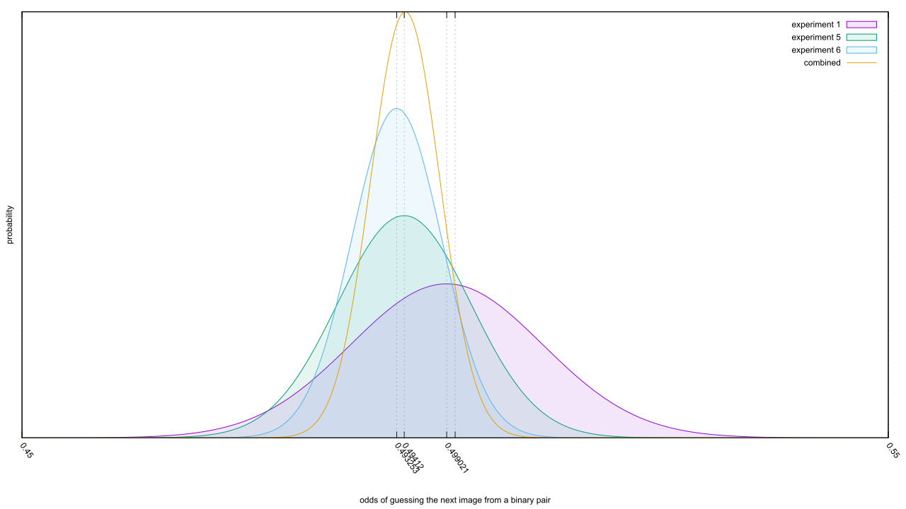
As the heading suggests, there’s something interesting hidden in the control groups. I’ll start with the binary image pair controls, which behave a lot like a coin flip; as the samples pile up, we’d expect the control distribution to migrate to the 50% line. When we do all the gathering, we find…

What happens when we combine the control groups for the binary image process from Bem (2011).… that’s not good. Experiment 1 had a great control group, but the controls from experiment 5 and 6 are oddly skewed. Since they had a lot more samples, they wind up dominating the posterior distribution and we find ourselves with fully 92.5% of the distribution below the expected value of p = 0.5. This sets up a bad precedent, because we now know that Bem’s methodology can create a skew of 0.67% away from 50%; for comparison, the combined signal from all studies was a skew of 0.83%. Are there bigger skews in the methodology of experiments 2, 3, 4, or 7? We’ve got no idea, because Bem never ran control groups.

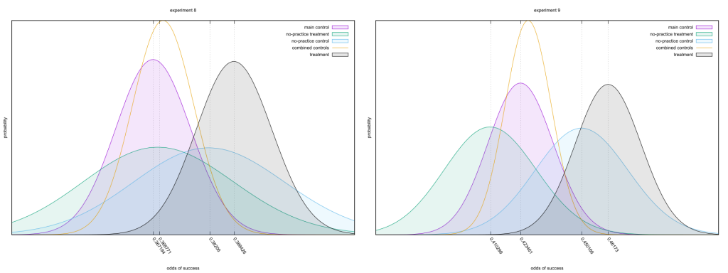
Experiments 3 and 4 lack any sort of control, so we’re left to consider the strongest pair of experiments in Bem’s paper, 8 and 9. Bem used a Differential Recall score instead of the raw guess count, as it makes the null effect have an expected value of zero. This Bayesian analysis can cope with a non-zero null, so I’ll just use a conventional success/failure count.

Experiments 8 and 9 from Bem's 2011 paper.

On the surface, everything’s on the up-and-up. The controls have more datapoints between them than the treatment group, but there’s good and consistent separation between them and the treatment. Look very careful at the numbers on the bottom, though; the effects are in quite different places. That’s strange, given the second study only differs from the first via some extra practice (page 14); I can see that improving up the main control and treatment groups, but why does it also drag along the no-practice groups? Either there aren’t enough samples here to get rid of random noise, which seems unlikely, or the methodology changed enough to spoil the replication.

Come to think of it, one of those controls isn’t exactly a control. I’ll let Bem explain the difference.

Participants were first shown a set of words and given a free recall test of those words. They were then given a set of practice exercises on a randomly selected subset of those words. The psi hypothesis was that the practice exercises would retroactively facilitate the recall of those words, and, hence, participants would recall more of the to-be-practiced words than the unpracticed words. […]

Although no control group was needed to test the psi hypothesis in this experiment, we ran 25 control sessions in which the computer again randomly selected a 24-word practice set but did not actually administer the practice exercises. These control sessions were interspersed among the experimental sessions, and the experimenter was uninformed as to condition. [page 13]

So the “no-practice treatment,” as I dubbed it in the charts, is actually a test of precognition! It happens to be a lousy one, as without a round of post-hoc practice to prepare subjects their performance should be poor. Nonetheless, we’d expect it to be as good or better than the matching controls. So why, instead, was it consistently worse? And not just a little worse, either; for experiment 9, it was as worse from its control as the main control was from its treatment group.

What it all Means

I know, I seems to be a touch obsessed with one social science paper. The reason has less to do with the paper than the context around it: you can make a good argument that the current reproducibility crisis is thanks to Bem. Take the words of E.J. Wagenmakers et al.

Instead of revising our beliefs regarding psi, Bem’s research should instead cause us to revise our beliefs on methodology: The field of psychology currently uses methodological and statistical strategies that are too weak, too malleable, and offer far too many opportunities for researchers to befuddle themselves and their peers. […]

We realize that the above flaws are not unique to the experiments reported by Bem (2011). Indeed, many studies in experimental psychology suffer from the same mistakes. However, this state of affairs does not exonerate the Bem experiments. Instead, these experiments highlight the relative ease with which an inventive researcher can produce significant results even when the null hypothesis is true. This evidently poses a significant problem for the field and impedes progress on phenomena that are replicable and important.

Wagenmakers, Eric–Jan, et al. “Why psychologists must change the way they analyze their data: the case of psi: comment on Bem (2011).” (2011): 426.

When it was pointed out Bayesian methods wiped away his results, Bem started doing Bayesian analysis. When others pointed out a meta-analysis could do the same, Bem did that too. You want open data? Bem was a hipster on that front, sharing his data around to interested researchers and now the public. He’s been pushing for replication, too, and in recent years has begun pre-registering studies to stem the garden of forking paths. Bem appears to be following the rules of science, to the letter.

I also know from bitter experience that any sufficiently large research project will run into data quality issues. But, now that I’ve looked at Bem’s raw data, I’m feeling hoodwinked. I expected a few isolated issues, but nothing on this scale. If Bem’s 2011 paper really is a type specimen for what’s wrong with the scientific method, as practiced, then it implies that most scientists are garbage at designing experiments and collecting data.

I’m not sure I can accept that.

How to Become a Radical

If I had a word of the week, it would be “radicalization.” Some of why the term is hot in my circles is due to offline conversations, some of it stems from yet another aggrieved white male engaging in terrorism, and some from yet another study confirms Trump voters were driven by bigotry (via fearing the loss of privilege that comes from giving up your superiority to promote equality).

Some just came in via Rebecca Watson, though, who pointed me to a fascinating study.

For example, a shift from ‘I’ to ‘We’ was found to reflect a change from an individual to a collective identity (…). Social status is also related to the extent to which first person pronouns are used in communication. Low-status individuals use ‘I’ more than high-status individuals (…), while high-status individuals use ‘we’ more often (…). This pattern is observed both in real life and on Internet forums (…). Hence, a shift from “I” to “we” may signal an individual’s identification with the group and a rise in status when becoming an accepted member of the group.

… I think you can guess what Step Two is. Walk away from the screen, find a pen and paper, write down your guess, then read the next paragraph.

The forum investigated here is one of the largest Internet forums in Sweden, called Flashback (…). The forum claims to work for freedom of speech. It has over one million users who, in total, write 15 000 to 20 000 posts every day. It is often criticized for being extreme, for example in being too lenient regarding drug related posts but also for being hostile in allowing denigrating posts toward groups such as immigrants, Jews, Romas, and feminists. The forum has many sub-forums and we investigate one of these, which focuses on immigration issues.

The total text data from the sub-forum consists of 964 Megabytes. The total amount of data includes 700,000 posts from 11th of July, 2004 until 25th of April, 2015.

How did you do? I don’t think you’ll need pen or paper to guess what these scientists saw in Step Three.

We expected and found changes in cues related to group identity formation and intergroup differentiation. Specifically, there was a significant decrease in the use of ‘I’ and a simultaneous increase in the use of ‘we’ and ‘they’. This has previously been related to group identity formation and differentiation to one or more outgroups (…). Increased usage of plural, and decreased frequency of singular, nouns have also been found in both normal, and extremist, group formations (…). There was a decrease in singular pronouns and a relative increase in collective pronouns. The increase in collective pronouns referred both to the ingroup (we) and to one or more outgroups (they). These results suggest a shift toward a collective identity among participants, and a stronger differentiation between the own group and the outgroup(s).

Brilliant! We’ve confirmed one way people become radicalized: by hanging around in forums devoted to “free speech,” the hate dumped on certain groups gradually creates an in-group/out-group dichotomy, bringing out the worst in us.

Unfortunately, there’s a problem with the staircase.

Categories Dictionaries Example words Mean r
Group differentiation First person singular I, my, me -.0103 ***
First person plural We, our, us .0115 ***
Third person plural They, them, their .0081 ***
Certainty Absolutely, sure .0016 NS

***p < .001. NS = not significant. n=11,751.

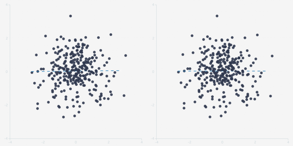
Table 2 tripped me up, hard. I dropped by the ever-awesome R<-Psychologist and cooked up two versions of the same dataset. One has no correlation, while the other has a correlation coefficient of 0.01. Can you tell me which is which, without resorting to a straight-edge or photo editor?

Comparing two datasets, one with r=0, the other with r=0.01.

I can’t either, because the effect size is waaaaaay too small to be perceptible. That’s a problem, because it can be trivially easy to manufacture a bias at least that large. If we were talking about a system with very tight constraints on its behaviour, like the Higgs Boson, then uncovering 500 bits of evidence over 2,500,000,000,000,000,000 trials could be too much for any bias to manufacture. But this study involves linguistics, which is far less precise than the Standard Model, so I need a solid demonstration of why this study is immune to biases on the scale of r = 0.01.

The authors do try to correct for how p-values exaggerate the evidence in large samples, but they do it by plucking p < 0.001 out of a hat. Not good enough; how does that p-value relate to studies of similar subject matter and methodology? Also, p-values stink. Also also, I notice there’s no control sample here. Do pro-social justice groups exhibit the same trend over time? What about the comment section of sports articles? It’s great that their hypotheses were supported by the data, don’t get me wrong, but it would be better if they’d tried harder to swat down their own hypothesis. I’d also like to point out that none of my complaints falsify their hypotheses, they merely demonstrate that the study falls well short of confirmed or significant, contrary to what I typed earlier.

Alas, I’ve discovered another path towards radicalization: perform honest research about the epistemology behind science. It’ll ruin your ability to read scientific papers, and leave you in despair about the current state of science.

Bayes Bunny iz trying to cool off after reading too many scientific papers.

One Hundred Prisoners

Here’s a question to puzzle out:

An especially cruel jailer announces a “game” to their 100 prisoners. A cabinet with 100 drawers sits in a heavily-monitored room. In each drawer lies one prisoner’s number. If every prisoner draws their own number from a drawer, every one of them walks free; if even one of them fails, however, all the prisoners must spend the rest of their days in solitary confinement. Prisoners must reset the drawers and room after their attempt, otherwise all of them head to solitary, and to ensure they cannot give each other hints everyone goes directly to solitary after their attempt. The jailer does offer a little mercy, though: prisoners can check up to half the drawers in the cabinet during their attempt, and collectively they have plenty of time to brainstorm a strategy.

What is the best one they could adopt?

This seems like a hopeless situation, no doubt. The odds of any one prisoner randomly finding their number is 50%, and the odds of that happening 100 times are so low they make death by shark look like a sure thing.

Nonetheless, the prisoners settle on a strategy. With a little programming code, we can evaluate the chances it’ll grant all their freedom.

      Algorithm	    Trials	      Successes	Percentage
   Random Guess	     50000	              0	0.0000000
         Cyclic	     50000	          15687	31.3740000

Whhaaa? How can the prisoners pull off odds like that? [Read more…]