[Content Warning: TERFs, high-level discussion of violence and sexual assault, math.]
[Content Warning: TERFs, high-level discussion of violence and sexual assault, math.]
Remember this old thing?
Rationality Rules was so confident nobody would take him to task, his “improved” video contains the same arguments as his “flawed” one. And honestly, he was right; I’ve seen this scenario play out often enough within this community to know that we try to bury our skeletons, that we treat our minorities like shit, that we “skeptics” are just as prone to being blind followers as the religious/woo crowds we critique. And just like all those other times, I cope by writing words until I get sick of the topic. Sometimes, that takes a while.
In hindsight, “a while” turned out to be seven months and about seventeen blog posts. Why on Earth would I spend so much time and effort focused on one vlogger? I don’t think I ever explained why in those posts, so let’s fix that: the atheist/skeptic movement has a problem with transphobia. From watching my peers insinuate Ann Coulter was a man, to my participation in l’affair Benson, I gradually went from “something feels off about this” to “wow, some of my peers are transphobes.”
As I picked apart the arguments made by transphobes, I started to see patterns. Much like with religious and alt-Right extremists, there’s a lot of recycling going on. Constantly, apologists are forced to search for new coats of paint to cover up old bigoted arguments. I spotted a shift from bathroom rhetoric to sports rhetoric in early 2019 and figured that approach would have a decent lifespan. So when Rationality Rules stuck to his transphobic guns, I took it as my opportunity to defuse sports-related transphobic arguments in general. If I did a good enough job, most of these posts would still be applicable when the next big-name atheist or skeptic tried to invoke sports.
My last post was a test of that. It was a draft I’d been nursing for months back in 2019, but after a fair bit of research and some drastic revisions I’d gotten Rationality Rules out of my system via other posts. So I set it aside as a test. If I truly was right about this shift to sports among transphobes, it was only a matter of time until someone else in the skeptic/atheist community would make a similar argument and some minor edits would make it relevant again. The upshot is that a handful of my readers were puzzled by this post about Rationality Rules, while the vast majority of you instead saw this post about Shermer and Shrier.
The two arguments aren’t quite the same. Rationality Rules emphasizes that “male puberty” is his dividing line; transgender women who start hormone therapy early enough can compete as women, according to him, and he relies on that to argue he’s not transphobic at all. Shermer is nowhere near as sophisticated, arguing for a new transgender-specific sporting category instead. Shrier takes the same stance as Rationality Rules, but she doesn’t push back on Shermer’s opinions.
But not only are the differences small, I doubt many people had “women are inherently inferior to men in domain X” on their transphobe bingo card. And yet, the same assertion was made at two very different times by three very different people. I consider this test a roaring success.
One consequence is that most of my prior posts on Rationality Rules’ arguments against transgender athletes still hold quite a bit of value, and are worth boosting. First, though, I should share the three relevant posts that got me interested in sports-related apologia:
Trans Athletes, the Existence of Gender Identity, … / … and Ophelia Benson: The first post proposed two high-level arguments in favour of allowing transgender athletes to compete as the gender they identify with. The second is mostly about calling out Benson for blatant misgendering, but I also debunk some irrational arguments made against transgender athletes.
I Think I Get It: My research for the prior two posts led me to flag sport inclusion as the next big thing in transphobic rhetoric. The paragraph claiming “they think of them as the worst of men” was written with Benson in mind, but was eerily predictive of Shermer.
And finally, the relevant Rationality Rules posts:
EssenceOfThought on Trans Athletes: This is mostly focused on EssenceOfThought‘s critique of Rationality Rules, but I slip in some extras relating to hemoglobin and testosterone.
Rationality Rules is an Oblivious Transphobe: My first crack at covering the primary factors of athletic performance (spoiler alert: nobody knows what they are) and the variation present. I also debunk some myths about transgender health care, refute some attempts to shift the burden of proof or argue evidence need not be provided.
Texas Sharpshooter: My second crack at athletic performance and its variance, this time with better analysis.
Rationality Rules is “A Transphobic Hack“: This is mostly commentary specific to Rationality Rules, but I do link to another EssenceOfThought video.
Special Pleading: My second crack at the human rights argument, correcting a mistake I made in another post.
Rationality Rules is a “Lying” Transphobe: I signal boost Rhetoric&Discourse‘s video on transgender athletes.
“Rationality Rules STILL Doesn’t Understand Sports”: A signal boost of Xevaris‘ video on transgender athletes.
Lies of Omission: Why the principle of “fair play” demands that transgender athletes be allowed to compete as their affirmed gender.
Begging the Question: How the term “male puberty” is transphobic.
Rationality Rules Is Delusional: Rob Clark directs me to a study that deflates the muscle fibre argument.
Cherry Picking: If transgender women possess an obvious performance benefit, you’d expect professional and amateur sporting bodies to reach a consensus on that benefit existing and to write their policies accordingly. Instead, they’re all over the place.
Separate and Unequal: I signal boost Colleen Tighe‘s comic on transgender athletes.
Rationality Rules DESTROYS Women’s Sport!!1!: I take a deep dive into a dataset on hormone levels in professional athletes, to see what would happen if we segregated sports by testosterone level. The title gives away the conclusion, alas.
That takes care of most of Shermer and Shrier’s arguments relating to transgender athletes, and the remainder should be pretty easy. I find it rather sad that neither are as skilled at transphobic arguments as Rationality Rules was. Is the atheist/skeptic community getting worse on this subject?
Sorry, sorry, got lost in my day job for a bit there. It’s been a month since the fundraising deadline passed, though, and I owe you some follow-up. So, the big question: did we hit the fundraising goal? Let’s load the dataset to find out. [Read more…]
TL;DR: We’re pretty much on track, though we also haven’t hit the goal of pushing the fund past $78,890.69. Donate and help put the fund over the line!
With the short version out of the way, let’s dive into the details. What’s changed in the past week and change?
import datetime as dt

import matplotlib.pyplot as pl

import pandas as pd
import pandas.tseries.offsets as pdto


cutoff_day = dt.datetime( 2020, 5, 27, tzinfo=dt.timezone(dt.timedelta(hours=-6)) )

donations = pd.read_csv('donations.cleaned.tsv',sep='\t')

donations['epoch'] = pd.to_datetime(donations['created_at'])
donations['delta_epoch'] = donations['epoch'] - cutoff_day
donations['delta_epoch_days'] = donations['delta_epoch'].apply(lambda x: x.days)

# some adjustment is necessary to line up with the current total
donations['culm'] = donations['amount'].cumsum() + 14723

new_donations_mask = donations['delta_epoch_days'] > 0
print( f"There have been {sum(new_donations_mask)} donations since {cutoff_day}." )
There have been 8 donations since 2020-05-27 00:00:00-06:00.
There’s been a reasonable number of donations after I published that original post. What does that look like, relative to the previous graph?
pl.figure(num=None, figsize=(8, 4), dpi=150, facecolor='w', edgecolor='k')

pl.plot( donations['delta_epoch_days'], donations['culm'], '-',c='#aaaaaa')
pl.plot( donations['delta_epoch_days'][new_donations_mask], \
        donations['culm'][new_donations_mask], '-',c='#0099ff')

pl.title("Defense against Carrier SLAPP Suit")

pl.xlabel("days since cutoff")
pl.ylabel("dollars")
pl.xlim( [-365.26,donations['delta_epoch_days'].max()] )
pl.ylim( [55000,82500] )
pl.show()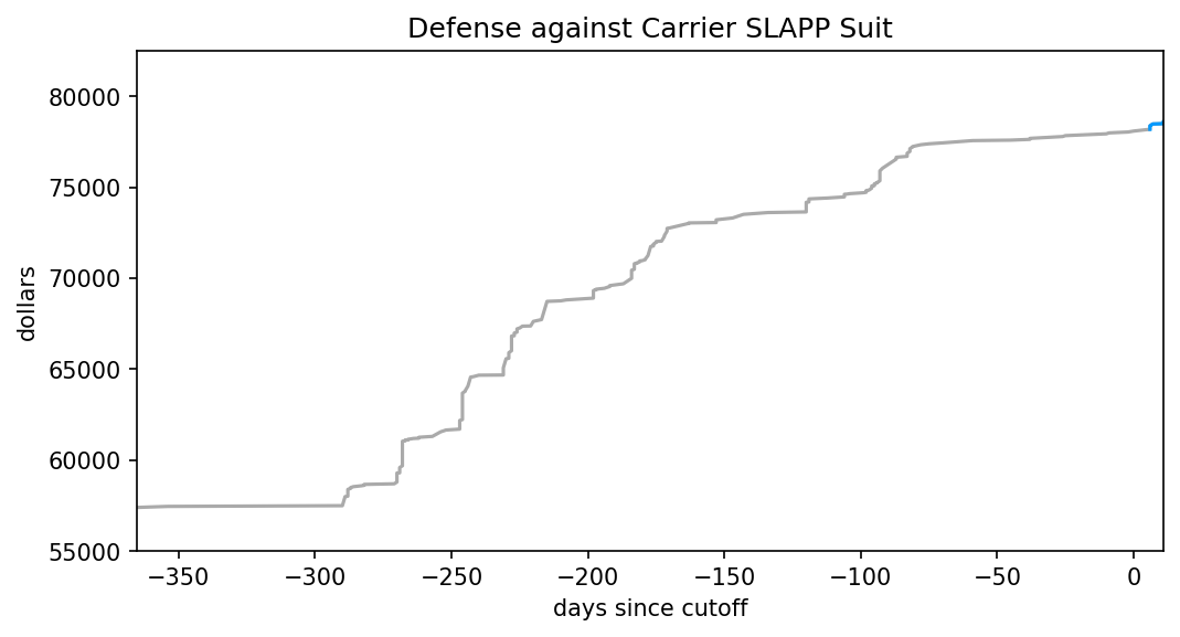
That’s certainly an improvement in the short term, though the graph is much too zoomed out to say more. Let’s zoom in, and overlay the posterior.
# load the previously-fitted posterior
flat_chain = np.loadtxt('starting_posterior.csv')


pl.figure(num=None, figsize=(8, 4), dpi=150, facecolor='w', edgecolor='k')

x = np.array([0, donations['delta_epoch_days'].max()])
for m,_,_ in flat_chain:
    pl.plot( x, m*x + 78039, '-r', alpha=0.05 )

pl.plot( donations['delta_epoch_days'], donations['culm'], '-', c='#aaaaaa')
pl.plot( donations['delta_epoch_days'][new_donations_mask], \
        donations['culm'][new_donations_mask], '-', c='#0099ff')

pl.title("Defense against Carrier SLAPP Suit")

pl.xlabel("days since cutoff")
pl.ylabel("dollars")
pl.xlim( [-3,x[1]+1] )
pl.ylim( [77800,79000] )

pl.show()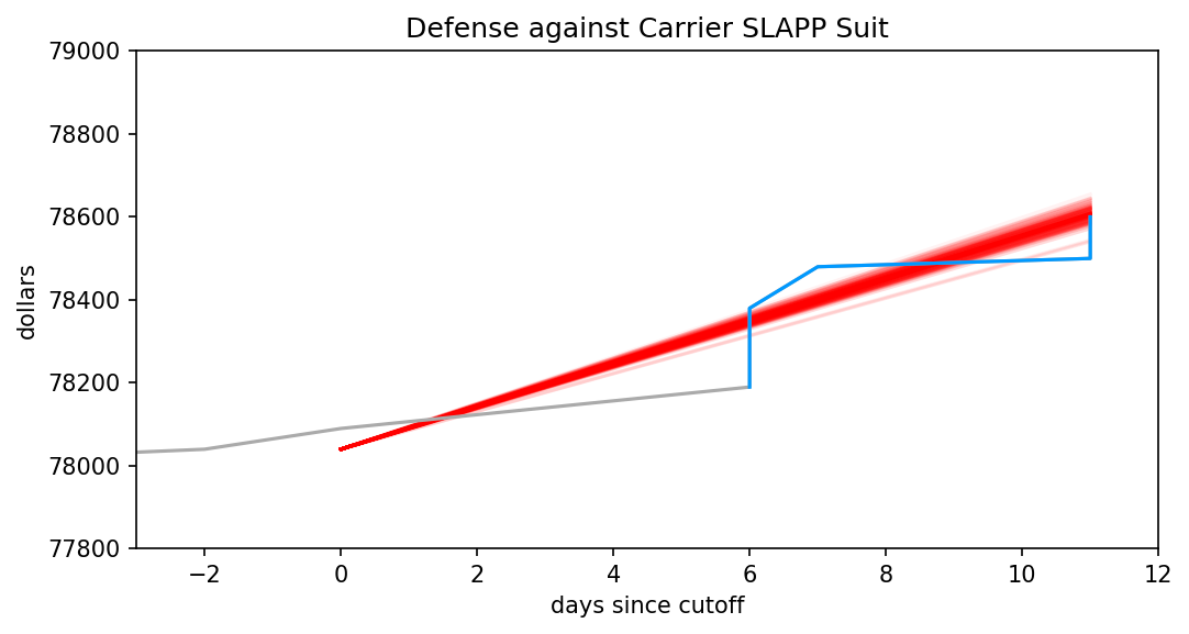
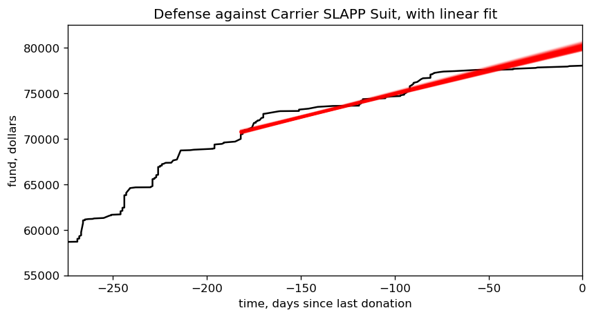
Hmm, looks like we’re right where the posterior predicted we’d be. My targets were pretty modest, though, consisting of an increase of 3% and 10%, so this doesn’t mean they’ve been missed. Let’s extend the chart to day 16, and explicitly overlay the two targets I set out.
low_target = 78890.69
high_target = 78948.57
target_day = dt.datetime( 2020, 6, 12, 23, 59, tzinfo=dt.timezone(dt.timedelta(hours=-6)) )
target_since_cutoff = (target_day - cutoff_day).days

pl.figure(num=None, figsize=(8, 4), dpi=150, facecolor='w', edgecolor='k')

x = np.array([0, target_since_cutoff])
pl.fill_between( x, [78039, low_target], [78039, high_target], color='#ccbbbb', label='blog post')
pl.fill_between( x, [78039, high_target], [high_target, high_target], color='#ffeeee', label='video')

pl.plot( donations['delta_epoch_days'], donations['culm'], '-',c='#aaaaaa')
pl.plot( donations['delta_epoch_days'][new_donations_mask], \
        donations['culm'][new_donations_mask], '-',c='#0099ff')

pl.title("Defense against Carrier SLAPP Suit")

pl.xlabel("days since cutoff")
pl.ylabel("dollars")
pl.xlim( [-3, target_since_cutoff] )
pl.ylim( [77800,high_target] )

pl.legend(loc='lower right')
pl.show()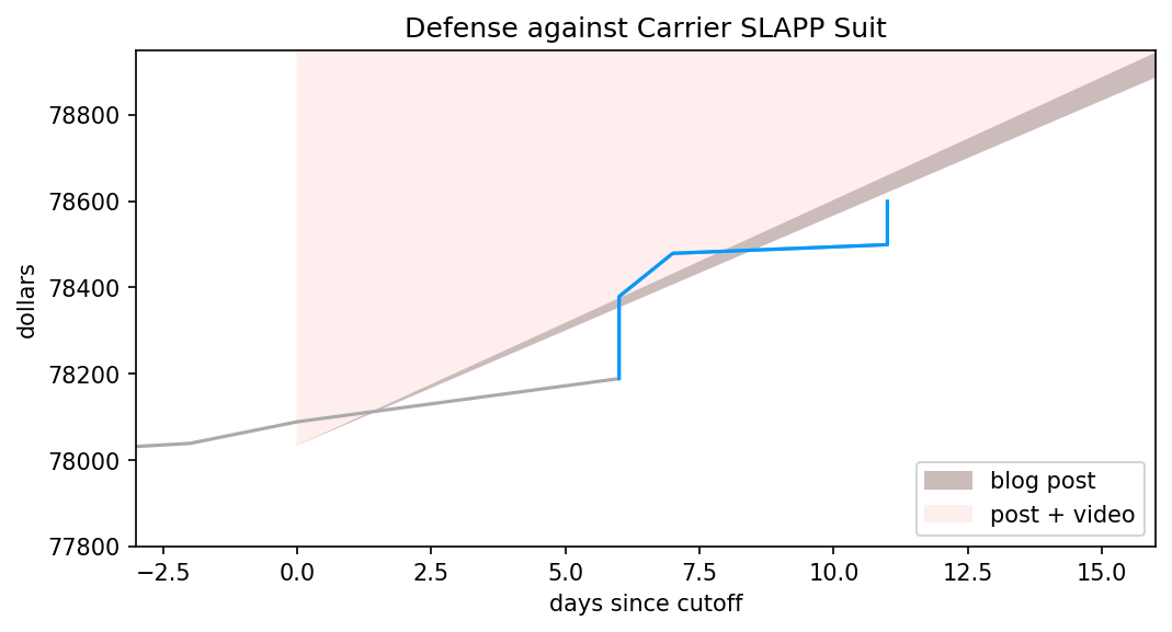
To earn a blog post and video on Bayes from me, we need the line to be in the pink zone by the time it reaches the end of the graph. For just the blog post, it need only be in the grayish- area. As you can see, it’s painfully close to being in line with the lower of two goals, though if nobody donates between now and Friday it’ll obviously fall quite short.
So if you want to see that blog post, get donating!
One of the ways I’m coping with this pandemic is studying it. Over the span of months I built up a list of questions specific to the situation in Alberta, so I figured I’d fire them off to the PR contact listed in one of the Alberta Government’s press releases.
That was a week ago. I haven’t even received an automated reply. I think it’s time to escalate this to the public sphere, as it might give those who can bend the government’s ear some idea of what they’re reluctant to answer. [Read more…]
If our goal is to raise funds for a good cause, we should at least have an idea of where the funds are at.
| created_at | amount | epoch | delta_epoch | culm | |
|---|---|---|---|---|---|
| 0 | 2017-01-24T07:27:51-06:00 | 10.0 | 2017-01-24 07:27:51-06:00 | -1218 days +19:51:12 | 14733.0 |
| 1 | 2017-01-24T07:31:09-06:00 | 50.0 | 2017-01-24 07:31:09-06:00 | -1218 days +19:54:30 | 14783.0 |
| 2 | 2017-01-24T07:41:20-06:00 | 100.0 | 2017-01-24 07:41:20-06:00 | -1218 days +20:04:41 | 14883.0 |
| 3 | 2017-01-24T07:50:20-06:00 | 10.0 | 2017-01-24 07:50:20-06:00 | -1218 days +20:13:41 | 14893.0 |
| 4 | 2017-01-24T08:03:26-06:00 | 25.0 | 2017-01-24 08:03:26-06:00 | -1218 days +20:26:47 | 14918.0 |
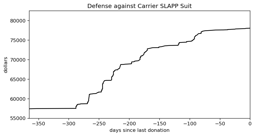
Changing the dataset so the last donation happens at time zero makes it both easier to fit the data and easier to understand what’s happening. The first day after the last donation is now day one.
Donations from 2017 don’t tell us much about the current state of the fund, though, so let’s focus on just the last year.
The donations seem to arrive in bursts, but there have been two quiet portions. One is thanks to the current pandemic, and the other was during last year’s late spring/early summer. It’s hard to tell what the donation rate is just by eye-ball, though. We need to smooth this out via a model.
The simplest such model is linear regression, aka. fitting a line. We want to incorporate uncertainty into the mix, which means a Bayesian fit. Now, what MCMC engine to use, hmmm…. emcee is my overall favourite, but I’m much too reliant on it. I’ve used PyMC3 a few times with success, but recently it’s been acting flaky. Time to pull out the big guns: Stan. I’ve been avoiding it because pystan‘s compilation times drove me nuts, but all the cool kids have switched to cmdstanpy when I looked away. Let’s give that a whirl.
CPU times: user 5.33 ms, sys: 7.33 ms, total: 12.7 ms
Wall time: 421 ms
CmdStan installed.
We can’t fit to the entire three-year time sequence, that just wouldn’t be fair given the recent slump in donations. How about the last six months? That covers both a few donation burts and a flat period, so it’s more in line with what we’d expect in future.
There were 117 donations over the last six months.
With the data prepped, we can shift to building the linear model.
I could have just gone with Stan’s basic model, but flat priors aren’t my style. My preferred prior for the slope is the inverse tangent, as it compensates for the tendency of large slope values to “bunch up” on one another. Stan doesn’t offer it by default, but the Cauchy distribution isn’t too far off.
We’d like the standard deviation to skew towards smaller values. It naturally tends to minimize itself when maximizing the likelihood, but an explicit skew will encourage this process along. Gelman and the Stan crew are drifting towards normal priors, but I still like a Cauchy prior for its weird properties.
Normally I’d plunk the Gaussian distribution in to handle divergence from the deterministic model, but I hear using Student’s T instead will cut down the influence of outliers. Thomas Wiecki recommends one degree of freedom, but Gelman and co. find that it leads to poor convergence in some cases. They recommend somewhere between three and seven degrees of freedom, but skew towards three, so I’ll go with the flow here.
The y-intercept could land pretty much anywhere, making its prior difficult to figure out. Yes, I’ve adjusted the time axis so that the last donation is at time zero, but the recent flat portion pretty much guarantees the y-intercept will be higher than the current amount of funds. The traditional approach is to use a flat prior for the intercept, and I can’t think of a good reason to ditch that.
Not convinced I picked good priors? That’s cool, there should be enough data here that the priors have minimal influence anyway. Moving on, let’s see how long compilation takes.
CPU times: user 4.91 ms, sys: 5.3 ms, total: 10.2 ms
Wall time: 20.2 s
This is one area where emcee really shines: as a pure python library, it has zero compilation time. Both PyMC3 and Stan need some time to fire up an external compiler, which adds overhead. Twenty seconds isn’t too bad, though, especially if it leads to quick sampling times.
CPU times: user 14.7 ms, sys: 24.7 ms, total: 39.4 ms
Wall time: 829 ms
And it does! emcee can be pretty zippy for a simple linear regression, but Stan is in another class altogether. PyMC3 floats somewhere between the two, in my experience.
Another great feature of Stan are the built-in diagnostics. These are really handy for confirming the posterior converged, and if not it can give you tips on what’s wrong with the model.
Processing csv files: /tmp/tmpyfx91ua9/linear_regression-202005262238-1-e393mc6t.csv, /tmp/tmpyfx91ua9/linear_regression-202005262238-2-8u_r8umk.csv, /tmp/tmpyfx91ua9/linear_regression-202005262238-3-m36dbylo.csv, /tmp/tmpyfx91ua9/linear_regression-202005262238-4-hxjnszfe.csv

Checking sampler transitions treedepth.
Treedepth satisfactory for all transitions.

Checking sampler transitions for divergences.
No divergent transitions found.

Checking E-BFMI - sampler transitions HMC potential energy.
E-BFMI satisfactory for all transitions.

Effective sample size satisfactory.

Split R-hat values satisfactory all parameters.

Processing complete, no problems detected.
The odds of a simple model with plenty of datapoints going sideways are pretty small, so this is another non-surprise. Enough waiting, though, let’s see the fit in action. First, we need to extract the posterior from the stored variables …
There are 256 samples in the posterior.
… and now free of its prison, we can plot the posterior against the original data. I’ll narrow the time window slightly, to make it easier to focus on the fit.
Looks like a decent fit to me, so we can start using it to answer a few questions. How much money is flowing into the fund each day, on average? How many years will it be until all those legal bills are paid off? Since humans aren’t good at counting in years, let’s also translate that number into a specific date.
mean/std/median slope = $51.62/1.65/51.76 per day

mean/std/median years to pay off the legal fees, relative to 2020-05-25 12:36:39-05:00 =
	1.962/0.063/1.955

mean/median estimate for paying off debt =
	2022-05-12 07:49:55.274942-05:00 / 2022-05-09 13:57:13.461426-05:00
Mid-May 2022, eh? That’s… not ideal. How much time can we shave off, if we increase the donation rate? Let’s play out a few scenarios.
median estimate for paying off debt, increasing rate by   1% = 2022-05-02 17:16:37.476652800
median estimate for paying off debt, increasing rate by   3% = 2022-04-18 23:48:28.185868800
median estimate for paying off debt, increasing rate by  10% = 2022-03-05 21:00:48.510403200
median estimate for paying off debt, increasing rate by  30% = 2021-11-26 00:10:56.277984
median estimate for paying off debt, increasing rate by 100% = 2021-05-17 18:16:56.230752
Bumping up the donation rate by one percent is pitiful. A three percent increase will almost shave off a month, which is just barely worthwhile, and a ten percent increase will roll the date forward by two. Those sound like good starting points, so let’s make them official: increase the current donation rate by three percent, and I’ll start pumping out the aforementioned blog posts on Bayesian statistics. Manage to increase it by 10%, and I’ll also record them as videos.
As implied, I don’t intend to keep the same rate throughout this entire process. If you surprise me with your generosity, I’ll bump up the rate. By the same token, though, if we go through a dry spell I’ll decrease the rate so the targets are easier to hit. My goal is to have at least a 50% success rate on that lower bar. Wouldn’t that make it impossible to hit the video target? Remember, though, it’ll take some time to determine the success rate. That lag should make it possible to blow past the target, and by the time this becomes an issue I’ll have thought of a better fix.
Ah, but over what timeframe should this rate increase? We could easily blow past the three percent target if someone donates a hundred bucks tomorrow, after all, and it’s no fair to announce this and hope your wallets are ready to go in an instant. How about… sixteen days. You’ve got sixteen days to hit one of those rate targets. That’s a nice round number, for a computer scientist, and it should (hopefully!) give me just enough time to whip up the first post. What does that goal translate to, in absolute numbers?
a 3% increase over 16 days translates to $851.69 + $78039.00 = $78890.69
Right, if you want those blog posts to start flowing you’ve got to get that fundraiser total to $78,890.69 before June 12th. As for the video…
a 10% increase over 16 days translates to $909.57 + $78039.00 = $78948.57
… you’ve got to hit $78,948.57 by the same date.
Ready? Set? Get donating!
I’ll admit, this fundraiser isn’t exactly twisting my arm. I’ve been mulling over how I’d teach Bayesian statistics for a few years. Overall, I’ve been most impressed with E.T. Jaynes’ approach, which draws inspiration from Cox’s Theorem. You’ll see a lot of similarities between my approach and Jaynes’, though I diverge on a few points. [Read more…]
I’m back! Yay! Sorry about all that, but my workload was just ridiculous. Things should be a lot more slack for the next few months, so it’s time I got back blogging. This also means I can finally put into action something I’ve been sitting on for months.
Richard Carrier has been a sore spot for me. He was one of the reasons I got interested in Bayesian statistics, and for a while there I thought he was a cool progressive. Alas, when it was revealed he was instead a vindictive creepy asshole, it shook me a bit. I promised myself I’d help out somehow, but I’d already done the obsessive analysis thing and in hindsight I’m not convinced it did more good than harm. I was at a loss for what I could do, beyond sharing links to the fundraiser.
Now, I think I know. The lawsuits may be long over, thanks to Carrier coincidentally dropping them at roughly the same time he came under threat of a counter-suit, but the legal bill are still there and not going away anytime soon. Worse, with the removal of the threat people are starting to forget about those debts. There have been only five donations this month, and four in April. It’s time to bring a little attention back that way.
One nasty side-effect of Carrier’s lawsuits is that Bayesian statistics has become a punchline in the atheist/skeptic community. The reasoning is understandable, if flawed: Carrier is a crank, he promotes Bayesian statistics, ergo Bayesian statistics must be the tool of crackpots. This has been surreal for me to witness, as Bayes has become a critical tool in my kit over the last three years. I suppose I could survive without it, if I had to, but every alternative I’m aware of is worse. I’m not the only one in this camp, either.
Following the emergence of a novel coronavirus (SARS-CoV-2) and its spread outside of China, Europe is now experiencing large epidemics. In response, many European countries have implemented unprecedented non-pharmaceutical interventions including case isolation, the closure of schools and universities, banning of mass gatherings and/or public events, and most recently, widescale social distancing including local and national lockdowns. In this report, we use a semi-mechanistic Bayesian hierarchical model to attempt to infer the impact of these interventions across 11 European countries.
Flaxman, Seth, Swapnil Mishra, Axel Gandy, H Juliette T Unwin, Helen Coupland, Thomas A Mellan, Tresnia Berah, et al. “Estimating the Number of Infections and the Impact of Non- Pharmaceutical Interventions on COVID-19 in 11 European Countries,” 2020, 35.In estimating time intervals between symptom onset and outcome, it was necessary to account for the fact that, during a growing epidemic, a higher proportion of the cases will have been infected recently (…). Therefore, we re-parameterised a gamma model to account for exponential growth using a growth rate of 0·14 per day, obtained from the early case onset data (…). Using Bayesian methods, we fitted gamma distributions to the data on time from onset to death and onset to recovery, conditional on having observed the final outcome.
Verity, Robert, Lucy C. Okell, Ilaria Dorigatti, Peter Winskill, Charles Whittaker, Natsuko Imai, Gina Cuomo-Dannenburg, et al. “Estimates of the Severity of Coronavirus Disease 2019: A Model-Based Analysis.” The Lancet Infectious Diseases 0, no. 0 (March 30, 2020). https://doi.org/10.1016/S1473-3099(20)30243-7.… we used Bayesian methods to infer parameter estimates and obtain credible intervals.
Linton, Natalie M., Tetsuro Kobayashi, Yichi Yang, Katsuma Hayashi, Andrei R. Akhmetzhanov, Sung-mok Jung, Baoyin Yuan, Ryo Kinoshita, and Hiroshi Nishiura. “Incubation Period and Other Epidemiological Characteristics of 2019 Novel Coronavirus Infections with Right Truncation: A Statistical Analysis of Publicly Available Case Data.” Journal of Clinical Medicine 9, no. 2 (February 2020): 538. https://doi.org/10.3390/jcm9020538.
A significant chunk of our understanding of COVID-19 depends on Bayesian statistics. I’ll go further and argue that you cannot fully understand this pandemic without it. And yet thanks to Richard Carrier, the atheist/skeptic community is primed to dismiss Bayesian statistics.
So let’s catch two stones with one bird. If enough people donate to this fundraiser, I’ll start blogging a course on Bayesian statistics. I think I’ve got a novel angle on the subject, one that’s easier to slip into than my 201-level stuff and yet more rigorous. If y’all really start tossing in the funds, I’ll make it a video series. Yes yes, there’s a pandemic and potential global depression going on, but that just means I’ll work for cheap! I’ll release the milestones and course outline over the next few days, but there’s no harm in an early start.
Help me help the people Richard Carrier hurt. I’ll try to make it worth your while.
Hello! I’ve been a fan of your work for some time. While I’ve used emcee more and currently use a lot of PyMC3, I love the layout of Stan‘s language and often find myself missing it.
But there’s no contradiction between being a fan and critiquing your work. And one of your recent blog posts left me scratching my head.
Suppose I want to estimate my chances of winning the lottery by buying a ticket every day. That is, I want to do a pure Monte Carlo estimate of my probability of winning. How long will it take before I have an estimate that’s within 10% of the true value?
This one’s pretty easy to set up, thanks to conjugate priors. The Beta distribution models our credibility of the odds of success from a Bernoulli process. If our prior belief is represented by the parameter pair \((\alpha_\text{prior},\beta_\text{prior})\), and we win \(w\) times over \(n\) trials, our posterior belief in the odds of us winning the lottery, \(p\), is
$$ \begin{align}
\alpha_\text{posterior} &= \alpha_\text{prior} + w, \\
\beta_\text{posterior} &= \beta_\text{prior} + n – w
\end{align} $$
You make it pretty clear that by “lottery” you mean the traditional kind, with a big payout that your highly unlikely to win, so \(w \approx 0\). But in the process you make things much more confusing.
There’s a big NY state lottery for which there is a 1 in 300M chance of winning the jackpot. Back of the envelope, to get an estimate within 10% of the true value of 1/300M will take many millions of years.
“Many millions of years,” when we’re “buying a ticket every day?” That can’t be right. The mean of the Beta distribution is
$$ \begin{equation}
\mathbb{E}[Beta(\alpha_\text{posterior},\beta_\text{posterior})] = \frac{\alpha_\text{posterior}}{\alpha_\text{posterior} + \beta_\text{posterior}}
\end{equation} $$
So if we’re trying to get that within 10% of zero, and \(w = 0\), we can write
$$ \begin{align}
\frac{\alpha_\text{prior}}{\alpha_\text{prior} + \beta_\text{prior} + n} &< \frac{1}{10} \\
10 \alpha_\text{prior} &< \alpha_\text{prior} + \beta_\text{prior} + n \\
9 \alpha_\text{prior} – \beta_\text{prior} &< n
\end{align} $$
If we plug in a sensible-if-improper subjective prior like \(\alpha_\text{prior} = 0, \beta_\text{prior} = 1\), then we don’t even need to purchase a single ticket. If we insist on an “objective” prior like Jeffrey’s, then we need to purchase five tickets. If for whatever reason we foolishly insist on the Bayes/Laplace prior, we need nine tickets. Even at our most pessimistic, we need less than a fortnight (or, if you prefer, much less than a Fortnite season). If we switch to the maximal likelihood instead of the mean, the situation gets worse.
$$ \begin{align}
\text{Mode}[Beta(\alpha_\text{posterior},\beta_\text{posterior})] &= \frac{\alpha_\text{posterior} – 1}{\alpha_\text{posterior} + \beta_\text{posterior} – 2} \\
\frac{\alpha_\text{prior} – 1}{\alpha_\text{prior} + \beta_\text{prior} + n – 2} &< \frac{1}{10} \\
9\alpha_\text{prior} – \beta_\text{prior} – 8 &< n
\end{align} $$
Now Jeffrey’s prior doesn’t require us to purchase a ticket, and even that awful Bayes/Laplace prior needs just one purchase. I can’t see how you get millions of years out of that scenario.
Maybe you meant a different scenario, though. We often use credible intervals to make decisions, so maybe you meant that the entire interval has to pass below the 0.1 mark? This introduces another variable, the width of the credible interval. Most people use two standard deviations or thereabouts, but I and a few others prefer a single standard deviation. Let’s just go with the higher bar, and start hacking away at the variance of the Beta distribution.
$$ \begin{align}
\text{var}[Beta(\alpha_\text{posterior},\beta_\text{posterior})] &= \frac{\alpha_\text{posterior}\beta_\text{posterior}}{(\alpha_\text{posterior} + \beta_\text{posterior})^2(\alpha_\text{posterior} + \beta_\text{posterior} + 2)} \\
\sigma[Beta(\alpha_\text{posterior},\beta_\text{posterior})] &= \sqrt{\frac{\alpha_\text{prior}(\beta_\text{prior} + n)}{(\alpha_\text{prior} + \beta_\text{prior} + n)^2(\alpha_\text{prior} + \beta_\text{prior} + n + 2)}} \\
\frac{\alpha_\text{prior}}{\alpha_\text{prior} + \beta_\text{prior} + n} + \frac{2}{\alpha_\text{prior} + \beta_\text{prior} + n} \sqrt{\frac{\alpha_\text{prior}(\beta_\text{prior} + n)}{\alpha_\text{prior} + \beta_\text{prior} + n + 2}} &< \frac{1}{10}
\end{align} $$
Our improper subjective prior still requires zero ticket purchases, as \(\alpha_\text{prior} = 0\) wipes out the entire mess. For Jeffrey’s prior, we find
$$ \begin{equation}
\frac{\frac{1}{2}}{n + 1} + \frac{2}{n + 1} \sqrt{\frac{1}{2}\frac{n + \frac 1 2}{n + 3}} < \frac{1}{10},
\end{equation} $$
which needs 18 ticket purchases according to Wolfram Alpha. The awful Bayes/Laplace prior can almost get away with 27 tickets, but not quite. Both of those stretch the meaning of “back of the envelope,” but you can get the answer via a calculator and some trial-and-error.
I used the term “hacking” for a reason, though. That variance formula is only accurate when \(p \approx \frac 1 2\) or \(n\) is large, and neither is true in this scenario. We’re likely underestimating the number of tickets we’d need to buy. To get an accurate answer, we need to integrate the Beta distribution.
$$ \begin{align}
\int_{p=0}^{\frac{1}{10}} \frac{\Gamma(\alpha_\text{posterior} + \beta_\text{posterior})}{\Gamma(\alpha_\text{posterior})\Gamma(\beta_\text{posterior})} p^{\alpha_\text{posterior} – 1} (1-p)^{\beta_\text{posterior} – 1} > \frac{39}{40} \\
40 \frac{\Gamma(\alpha_\text{prior} + \beta_\text{prior} + n)}{\Gamma(\alpha_\text{prior})\Gamma(\beta_\text{prior} + n)} \int_{p=0}^{\frac{1}{10}} p^{\alpha_\text{prior} – 1} (1-p)^{\beta_\text{prior} + n – 1} > 39
\end{align} $$
Awful, but at least for our subjective prior it’s trivial to evaluate. \(\text{Beta}(0,n+1)\) is a Dirac delta at \(p = 0\), so 100% of the integral is below 0.1 and we still don’t need to purchase a single ticket. Fortunately for both the Jeffrey’s and Bayes/Laplace prior, my “envelope” is a Jupyter notebook.
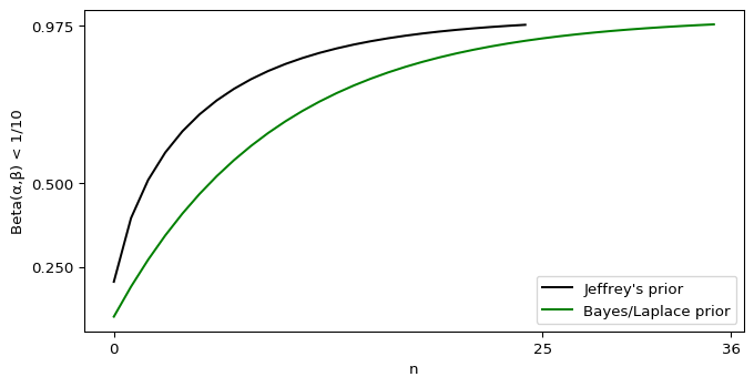
Those numbers did go up by a non-trivial amount, but we’re still nowhere near “many millions of years,” even if Fortnite’s last season felt that long.
Maybe you meant some scenario where the credible interval overlaps \(p = 0\)? With proper priors, that never happens; the lower part of the credible interval always leaves room for some extremely small values of \(p\), and thus never actually equals 0. My sensible improper prior has both ends of the interval equal to zero and thus as long as \(w = 0\) it will always overlap \(p = 0\).
I think I can find a scenario where you’re right, but I also bet you’re sick of me calling \((0,1)\) a “sensible” subjective prior. Hope you don’t mind if I take a quick detour to the last question in that blog post, which should explain how a Dirac delta can be sensible.
How long would it take to convince yourself that playing the lottery has an expected negative return if tickets cost $1, there’s a 1/300M chance of winning, and the payout is $100M?
Let’s say the payout if you win is \(W\) dollars, and the cost of a ticket is \(T\). Then your expected earnings at any moment is an integral of a multiple of the entire Beta posterior.
$$ \begin{equation}
\mathbb{E}(\text{Lottery}_{W}) = \int_{p=0}^1 \frac{\Gamma(\alpha_\text{posterior} + \beta_\text{posterior})}{\Gamma(\alpha_\text{posterior})\Gamma(\beta_\text{posterior})} p^{\alpha_\text{posterior} – 1} (1-p)^{\beta_\text{posterior} – 1} p W < T
\end{equation} $$
I’m pretty confident you can see why that’s a back-of-the-envelope calculation, but this is a public letter and I’m also sure some of those readers just fainted. Let me detour from the detour to assure them that, yes, this is actually a pretty simple calculation. They’ve already seen that multiplicative constants can be yanked out of the integral, but I’m not sure they realized that if
$$ \begin{equation}
\int_{p=0}^1 \frac{\Gamma(\alpha + \beta)}{\Gamma(\alpha)\Gamma(\beta)} p^{\alpha – 1} (1-p)^{\beta – 1} = 1,
\end{equation} $$
then thanks to the multiplicative constant rule it must be true that
$$ \begin{equation}
\int_{p=0}^1 p^{\alpha – 1} (1-p)^{\beta – 1} = \frac{\Gamma(\alpha)\Gamma(\beta)}{\Gamma(\alpha + \beta)}
\end{equation} $$
They may also be unaware that the Gamma function is an analytic continuity of the factorial. I say “an” because there’s an infinite number of functions that also qualify. To be considered a “good” analytic continuity the Gamma function must also duplicate another property of the factorial, that \((a + 1)! = (a + 1)(a!)\) for all valid \(a\). Or, put another way, it must be true that
$$ \begin{equation}
\frac{\Gamma(a + 1)}{\Gamma(a)} = a + 1, a > 0
\end{equation} $$
Fortunately for me, the Gamma function is a good analytic continuity, perhaps even the best. This allows me to chop that integral down to size.
$$ \begin{align}
W \frac{\Gamma(\alpha_\text{prior} + \beta_\text{prior} + n)}{\Gamma(\alpha_\text{prior})\Gamma(\beta_\text{prior} + n)} \int_{p=0}^1 p^{\alpha_\text{prior} – 1} (1-p)^{\beta_\text{prior} + n – 1} p &< T \\
\int_{p=0}^1 p^{\alpha_\text{prior} – 1} (1-p)^{\beta_\text{prior} + n – 1} p &= \int_{p=0}^1 p^{\alpha_\text{prior}} (1-p)^{\beta_\text{prior} + n – 1} \\
\int_{p=0}^1 p^{\alpha_\text{prior}} (1-p)^{\beta_\text{prior} + n – 1} &= \frac{\Gamma(\alpha_\text{prior} + 1)\Gamma(\beta_\text{prior} + n)}{\Gamma(\alpha_\text{prior} + \beta_\text{prior} + n + 1)} \\
W \frac{\Gamma(\alpha_\text{prior} + \beta_\text{prior} + n)}{\Gamma(\alpha_\text{prior})\Gamma(\beta_\text{prior} + n)} \frac{\Gamma(\alpha_\text{prior} + 1)\Gamma(\beta_\text{prior} + n)}{\Gamma(\alpha_\text{prior} + \beta_\text{prior} + n + 1)} &< T \\
W \frac{\Gamma(\alpha_\text{prior} + \beta_\text{prior} + n) \Gamma(\alpha_\text{prior} + 1)}{\Gamma(\alpha_\text{prior} + \beta_\text{prior} + n + 1) \Gamma(\alpha_\text{prior})} &< T \\
W \frac{\alpha_\text{prior} + 1}{\alpha_\text{prior} + \beta_\text{prior} + n + 1} &< T \\
\frac{W}{T}(\alpha_\text{prior} + 1) – \alpha_\text{prior} – \beta_\text{prior} – 1 &< n
\end{align} $$
Mmmm, that was satisfying. Anyway, for Jeffrey’s prior you need to purchase \(n > 149,999,998\) tickets to be convinced this lottery isn’t worth investing in, while the Bayes/Laplace prior argues for \(n > 199,999,997\) purchases. Plug my subjective prior in, and you’d need to purchase \(n > 99,999,998\) tickets.
That’s optimal, assuming we know little about the odds of winning this lottery. The number of tickets we need to purchase is controlled by our prior. Since \(W \gg T\), our best bet to minimize the number of tickets we need to purchase is to minimize \(\alpha_\text{prior}\). Unfortunately, the lowest we can go is \(\alpha_\text{prior} = 0\). Almost all the “objective” priors I know of have it larger, and thus ask that you sink more money into the lottery than the prize is worth. That doesn’t sit well with our intuition. The sole exception is the Haldane prior of (0,0), which argues for \(n > 99,999,999\) and thus asks you to spend exactly as much as the prize-winnings. By stating \(\beta_\text{prior} = 1\), my prior manages to shave off one ticket purchase.
Another prior that increases \(\beta_\text{prior}\) further will shave off further purchases, but so far we’ve only considered the case where \(w = 0\). What if we sink money into this lottery, and happen to win before hitting our limit? The subjective prior of \((0,1)\) after \(n\) losses becomes equivalent to the Bayes/Laplace prior of \((1,1)\) after \(n-1\) losses. Our assumption that \(p \approx 0\) has been proven wrong, so the next best choice is to make no assumptions about \(p\). At the same time, we’ve seen \(n\) losses and we’d be foolish to discard that information entirely. A subjective prior with \(\beta_\text{prior} > 1\) wouldn’t transform in this manner, while one with \(\beta_\text{prior} < 1\) would be biased towards winning the lottery relative to the Bayes/Laplace prior.
My subjective prior argues you shouldn’t play the lottery, which matches the reality that almost all lotteries pay out less than they take in, but if you insist on participating it will minimize your losses while still responding well to an unexpected win. It lives up to the hype.
However, there is one way to beat it. You mentioned in your post that the odds of winning this lottery are one in 300 million. We’re not supposed to incorporate that into our math, it’s just a measuring stick to use against the values we churn out, but what if we constructed a prior around it anyway? This prior should have a mean of one in 300 million, and the \(p = 0\) case should have zero likelihood. The best match is \((1+\epsilon, 299999999\cdot(1+\epsilon))\), where \(\epsilon\) is a small number, and when we take a limit …
$$ \begin{equation}
\lim_{\epsilon \to 0^{+}} \frac{100,000,000}{1}(2 + \epsilon) – 299,999,999 \epsilon – 300,000,000 = -100,000,000 < n
\end{equation} $$
… we find the only winning move is not to play. There’s no Dirac deltas here, either, so unlike my subjective prior it’s credible interval is one-dimensional. Eliminating the \(p = 0\) case runs contrary to our intuition, however. A newborn that purchased a ticket every day of its life until it died on its 80th birthday has a 99.99% chance of never holding a winning ticket. \(p = 0\) is always an option when you live a finite amount of time.
The problem with this new prior is that it’s incredibly strong. If we didn’t have the true odds of winning in our back pocket, we could quite fairly be accused of putting our thumb on the scales. We can water down \((1,299999999)\) by dividing both \(\alpha_\text{prior}\) and \(\beta_\text{prior}\) by a constant value. This maintains the mean of the Beta distribution, and while the \(p = 0\) case now has non-zero credence I’ve shown that’s no big deal. Pick the appropriate constant value and we get something like \((\epsilon,1)\), where \(\epsilon\) is a small positive value. Quite literally, that’s within epsilon of the subjective prior I’ve been hyping!
So far, the only back-of-the-envelope calculations I’ve done that argued for millions of ticket purchases involved the expected value, but that was only because we used weak priors that are a poor match for reality. I believe in the principle of charity, though, and I can see a scenario where a back-of-the-envelope calculation does demand millions of purchases.
But to do so, I’ve got to hop the fence and become a frequentist.
If you haven’t read The Theory That Would Not Die, you’re missing out. Sharon Bertsch McGrayne mentions one anecdote about the RAND Corporation’s attempts to calculate the odds of a nuclear weapon accidentally detonating back in the 1950’s. No frequentist statistician would touch it with a twenty-foot pole, but not because they were worried about getting the math wrong. The problem was the math. As the eventually-published report states:
The usual way of estimating the probability of an accident in a given situation is to rely on observations of past accidents. This approach is used in the Air Force, for example, by the Directory of Flight Safety Research to estimate the probability per flying hour of an aircraft accident. In cases of of newly introduced aircraft types for which there are no accident statistics, past experience of similar types is used by analogy.
Such an approach is not possible in a field where this is no record of past accidents. After more than a decade of handling nuclear weapons, no unauthorized detonation has occurred. Furthermore, one cannot find a satisfactory analogy to the complicated chain of events that would have to precede an unauthorized nuclear detonation. (…) Hence we are left with the banal observation that zero accidents have occurred. On this basis the maximal likelihood estimate of the probability of an accident in any future exposure turns out to be zero.
For the lottery scenario, a frequentist wouldn’t reach for the Beta distribution but instead the Binomial. Given \(n\) trials of a Bernoulli process with probability \(p\) of success, the expected number of successes observed is
$$ \begin{equation}
\bar w = n p
\end{equation} $$
We can convert that to a maximal likelihood estimate by dividing the actual number of observed successes by \(n\).
$$ \begin{equation}
\hat p = \frac{w}{n}
\end{equation} $$
In many ways this estimate can be considered optimal, as it is both unbiased and has the least variance of all other estimators. Thanks to the Central Limit Theorem, the Binomial distribution will approximate a Gaussian distribution to arbitrary degree as we increase \(n\), which allows us to apply the analysis from the latter to the former. So we can use our maximal likelihood estimate \(\hat p\) to calculate the standard error of that estimate.
$$ \begin{equation}
\text{SEM}[\hat p] = \sqrt{ \frac{\hat p(1- \hat p)}{n} }
\end{equation} $$
Ah, but what if \(w = 0\)? It follows that \(\hat p = 0\), but this also means that \(\text{SEM}[\hat p] = 0\). There’s no variance in our estimate? That can’t be right. If we approach this from another angle, plugging \(w = 0\) into the Binomial distribution, it reduces to
$$ \begin{equation}
\text{Binomial}(w | n,p) = \frac{n!}{w!(n-w)!} p^w (1-p)^{n-w} = (1-p)^n
\end{equation} $$
The maximal likelihood of this Binomial is indeed \(p = 0\), but it doesn’t resemble a Dirac delta at all.
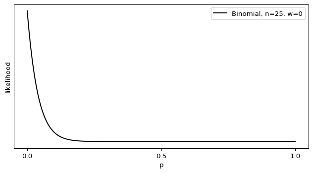
Shouldn’t there be some sort of variance there? What’s going wrong?
We got a taste of this on the Bayesian side of the fence. Using the stock formula for the variance of the Beta distribution underestimated the true value, because the stock formula assumed \(p \approx \frac 1 2\) or a large \(n\). When we assume we have a near-infinite amount of data, we can take all sorts of computational shortcuts that make our life easier. One look at the Binomial’s mean, however, tells us that we can drown out the effects of a large \(n\) with a small value of \(p\). And, just as with the odds of a nuclear bomb accident, we already know \(p\) is very, very small. That isn’t fatal on its own, as you correctly point out.
With the lottery, if you run a few hundred draws, your estimate is almost certainly going to be exactly zero. Did we break the [*Central Limit Theorem*]? Nope. Zero has the right absolute error properties. It’s within 1/300M of the true answer after all!
The problem comes when we apply the Central Limit Theorem and use a Gaussian approximation to generate a confidence or credible interval for that maximal likelihood estimate. As both the math and graph show, though, the probability distribution isn’t well-described by a Gaussian distribution. This isn’t much of a problem on the Bayesian side of the fence, as I can juggle multiple priors and switch to integration for small values of \(n\). Frequentism, however, is dependent on the Central Limit Theorem and thus assumes \(n\) is sufficiently large. This is baked right into the definitions: a p-value is the fraction of times you calculate a test metric equal to or more extreme than the current one assuming the null hypothesis is true and an infinite number of equivalent trials of the same random process, while confidence intervals are a range of parameter values such that when we repeat the maximal likelihood estimate on an infinite number of equivalent trials the estimates will fall in that range more often than a fraction of our choosing. Frequentist statisticians are stuck with the math telling them that \(p = 0\) with absolute certainty, which conflicts with our intuitive understanding.
For a frequentist, there appears to be only one way out of this trap: witness a nuclear bomb accident. Once \(w > 0\), the math starts returning values that better match intuition. Likewise with the lottery scenario, the only way for a frequentist to get an estimate of \(p\) that comes close to their intuition is to purchase tickets until they win at least once.
This scenario does indeed take “many millions of years.” It’s strange to find you taking a frequentist world-view, though, when you’re clearly a Bayesian. By straddling the fence you wind up in a world of hurt. For instance, you state this:
Did we break the [*Central Limit Theorem*]? Nope. Zero has the right absolute error properties. It’s within 1/300M of the true answer after all! But it has terrible relative error probabilities; it’s relative error after a lifetime of playing the lottery is basically infinity.
A true frequentist would have been fine asserting the probability of a nuclear bomb accident is zero. Why? Because \(\text{SEM}[\hat p = 0]\) is actually a very good confidence interval. If we’re going for two sigmas, then our confidence interval should contain the maximal likelihood we’ve calculated at least 95% of the time. Let’s say our sample sizes are \(n = 36\), the worst-case result from Bayesian statistics. If the true odds of winning the lottery are 1 in 300 million, then the odds of calculating a maximal likelihood of \(p = 0\) is
p( MLE(hat p) = 0 ) = 0.999999880000007
About 99.99999% of the time, then, the confidence interval of \(0 \leq \hat p \leq 0\) will be correct. That’s substantially better than 95%! Nothing’s broken here, frequentism is working exactly as intended.
I bet you think I’ve screwed up the definition of confidence intervals. I’m afraid not, I’ve double-checked my interpretation by heading back to the source, Jerzy Neyman. He, more than any other person, is responsible for pioneering the frequentist confidence interval.
We can then tell the practical statistician that whenever he is certain that the form of the probability law of the X’s is given by the function? \(p(E|\theta_1, \theta_2, \dots \theta_l,)\) which served to determine \(\underline{\theta}(E)\) and \(\bar \theta(E)\) [the lower and upper bounds of the confidence interval], he may estimate \(\theta_1\) by making the following three steps: (a) he must perform the random experiment and observe the particular values \(x_1, x_2, \dots x_n\) of the X’s; (b) he must use these values to calculate the corresponding values of \(\underline{\theta}(E)\) and \(\bar \theta(E)\); and (c) he must state that \(\underline{\theta}(E) < \theta_1^o < \bar \theta(E)\), where \(\theta_1^o\) denotes the true value of \(\theta_1\). How can this recommendation be justified?
[Neyman keeps alternating between \(\underline{\theta}(E) \leq \theta_1^o \leq \bar \theta(E)\) and \(\underline{\theta}(E) < \theta_1^o < \bar \theta(E)\) throughout this paper, so presumably both forms are A-OK.]
The justification lies in the character of probabilities as used here, and in the law of great numbers. According to this empirical law, which has been confirmed by numerous experiments, whenever we frequently and independently repeat a random experiment with a constant probability, \(\alpha\), of a certain result, A, then the relative frequency of the occurrence of this result approaches \(\alpha\). Now the three steps (a), (b), and (c) recommended to the practical statistician represent a random experiment which may result in a correct statement concerning the value of \(\theta_1\). This result may be denoted by A, and if the calculations leading to the functions \(\underline{\theta}(E)\) and \(\bar \theta(E)\) are correct, the probability of A will be constantly equal to \(\alpha\). In fact, the statement (c) concerning the value of \(\theta_1\) is only correct when \(\underline{\theta}(E)\) falls below \(\theta_1^o\) and \(\bar \theta(E)\), above \(\theta_1^o\), and the probability of this is equal to \(\alpha\) whenever \(\theta_1^o\) the true value of \(\theta_1\). It follows that if the practical statistician applies permanently the rules (a), (b) and (c) for purposes of estimating the value of the parameter \(\theta_1\) in the long run he will be correct in about 99 per cent of all cases. […]
It will be noticed that in the above description the probability statements refer to the problems of estimation with which the statistician will be concerned in the future. In fact, I have repeatedly stated that the frequency of correct results tend to \(\alpha\). [Footnote: This, of course, is subject to restriction that the X’s considered will follow the probability law assumed.] Consider now the case when a sample, E’, is already drawn and the calculations have given, say, \(\underline{\theta}(E’)\) = 1 and \(\bar \theta(E’)\) = 2. Can we say that in this particular case the probability of the true value of \(\theta_1\) falling between 1 and 2 is equal to \(\alpha\)?
The answer is obviously in the negative. The parameter \(\theta_1\) is an unknown constant and no probability statement concerning its value may be made, that is except for the hypothetical and trivial ones … which we have decided not to consider.
Neyman, Jerzy. “X — outline of a theory of statistical estimation based on the classical theory of probability.” Philosophical Transactions of the Royal Society of London. Series A, Mathematical and Physical Sciences 236.767 (1937): 348-349.
If there was any further doubt, it’s erased when Neyman goes on to analogize scientific measurements to a game of roulette. Just as the knowing where the ball landed doesn’t tell us anything about where the gamblers placed their bets, “once the sample \(E’\) is drawn and the values of \(\underline{\theta}(E’)\) and \(\bar \theta(E’)\) determined, the calculus of probability adopted here is helpless to provide answer to the question of what is the true value of \(\theta_1\).” (pg. 350)
If a confidence interval doesn’t tell us anything about where the true parameter value lies, then its only value must come from being an estimator of long-term behaviour. And as I showed before, \(\text{SEM}[\hat p = 0]\) estimates the maximal likelihood from repeating the experiment extremely well. It is derived from the long-term behaviour of the Binomial distribution, which is the correct distribution to describe this situation within frequentism. \(\text{SEM}[\hat p = 0]\) fits Neyman’s definition of a confidence interval perfectly, and thus generates a valid frequentist confidence interval. On the Bayesian side, I’ve spilled a substantial number of photons to convince you that a Dirac delta prior is a good choice, and that prior also generates zero-width credence intervals. If it worked over there, why can’t it also work over here?
This is Jayne’s Truncated Interval all over again. The rules of frequentism don’t work the way we intuit, which normally isn’t a problem because the Central Limit Theorem massages the data enough to align frequentism and intuition. Here, though, we’ve stumbled on a corner case where \(p = 0\) with absolute certainty and \(p \neq 0\) with tight error bars are both correct conclusions under the rules of frequentism. RAND Corporation should not have had any difficulty finding a frequentist willing to calculate the odds of a nuclear bomb accident, because they could have scribbled out one formula on an envelope and concluded such accidents were impossible.
And yet, faced with two contradictory answers or unaware the contradiction exists, frequentists side with intuition and reject the rules of their own statistical system. They strike off the \(p = 0\) answer, leaving only the case where \(p \ne 0\) and \(w > 0\). Since reality currently insists that \(w = 0\), they’re prevented from coming to any conclusion. The same reasoning leads to the “many millions of years” of ticket purchases that you argued was the true back-of-the-envelope conclusion. To break out of this rut, RAND Corporation was forced to abandon frequentism and instead get their estimate via Bayesian statistics.
On this basis the maximal likelihood estimate of the probability of an accident in any future exposure turns out to be zero. Obviously we cannot rest content with this finding. […]
… we can use the following idea: in an operation where an accident seems to be possible on technical grounds, our assurance that this operation will not lead to an accident in the future increases with the number of times this operation has been carried out safely, and decreases with the number of times it will be carried out in the future. Statistically speaking, this simple common sense idea is based on the notion that there is an a priori distribution of the probability of an accident in a given opportunity, which is not all concentrated at zero. In Appendix II, Section 2, alternative forms for such an a priori distribution are discussed, and a particular Beta distribution is found to be especially useful for our purposes.
It’s been said that frequentists are closet Bayesians. Through some misunderstandings and bad luck on your end, you’ve managed to be a Bayesian that’s a closet frequentist that’s a closet Bayesian. Had you stuck with a pure Bayesian view, any back-of-the-envelope calculation would have concluded that your original scenario demanded, in the worst case, that you’d need to purchase lottery tickets for a Fortnite.
I still can’t believe this post exists, given its humble beginnings.
The “women’s category” is, in my opinion, poorly named given our current climate, and so I’d elect a name more along the lines of the “Under 5 nmol/l category” (as in, under 5 nanomoles of testosterone per litre), but make no mistake about it, the “woman’s category” is not based on gender or identity, or even genitalia or chromosomes… it’s based on hormone levels and the absence of male puberty.
The above comment wasn’t in Rationality Rules’ latest transphobic video, it was just a casual aside by RR himself in the YouTube comment section. He’s obiquely doubled-down via Twitter (hat tip to Essence of Thought):
Of course, just as I support trans men competing in all “men’s categories” (poorly named), women who have not experienced male puberty competing in all women’s sport (also poorly named) and trans women who have experienced male puberty competing in long-distance running.
To further clarify, I think that we must rename our categories according to what they’re actually based on. It’s not right to have a “women’s category” and yet say to some trans women (who are women!) that they can’t compete within it; it should be renamed.
The proposal itched away at me, though, because I knew it was testable.
There is a need to clarify hormone profiles that may be expected to occur after competition when antidoping tests are usually made. In this study, we report on the hormonal profile of 693 elite athletes, sampled within 2 h of a national or international competitive event. These elite athletes are a subset of the cross-sectional study that was a component of the GH-2000 research project aimed at developing a test to detect abuse with growth hormone.
Healy, Marie-Louise, et al. “Endocrine profiles in 693 elite athletes in the postcompetition setting.” Clinical endocrinology 81.2 (2014): 294-305.
The GH-2000 project had already done the hard work of collecting and analyzing blood samples from athletes, so checking RR’s proposal was no tougher than running some numbers. There’s all sorts of ethical guidelines around sharing medical info, but fortunately there’s an easy shortcut: ask one of the scientists involved to run the numbers for me, and report back the results. Aggregate data is much more resistant to de-anonymization, so the ethical concerns are greatly reduced. The catch, of course, is that I’d have to find a friendly researcher with access to that dataset. About a month ago, I fired off some emails and hoped for the best.
I wound up much, much better than the best. I got full access to the dataset!! You don’t get handed an incredible gift like this and merely use it for a blog post. In my spare time, I’m flexing my Bayesian muscles to do a re-analysis of the above paper, while also looking for observations the original authors may have missed. Alas, that means my slow posting schedule is about to crawl.
But in the meantime, we have a question to answer.
Total Assigned-female Athletes = 239
  Height, Mean           = 171.61 cm
  Height, Std.Dev        = 7.12 cm
  Weight, Mean           = 64.27 kg
  Weight, Std.Dev        = 9.12 kg
  Body Fat, Mean         = 13.19 kg
  Body Fat, Std.Dev      = 3.85 kg
  Testosterone, Mean     = 2.68 nmol/L
  Testosterone, Std.Dev  = 4.33 nmol/L
  Testosterone, Max      = 31.90 nmol/L
  Testosterone, Min      = 0.00 nmol/L

Total Assigned-male Athletes = 454
  Height, Mean           = 182.72 cm
  Height, Std.Dev        = 8.48 cm
  Weight, Mean           = 80.65 kg
  Weight, Std.Dev        = 12.62 kg
  Body Fat, Mean         = 8.89 kg
  Body Fat, Std.Dev      = 7.20 kg
  Testosterone, Mean     = 14.59 nmol/L
  Testosterone, Std.Dev  = 6.66 nmol/L
  Testosterone, Max      = 41.00 nmol/L
  Testosterone, Min      = 0.80 nmol/L
The first step is to get a basic grasp on what’s there, via some crude descriptive statistics. It’s also useful to compare these with the original paper, to make sure I’m interpreting the data correctly. Excusing some minor differences in rounding, the above numbers match the paper.
The only thing that stands out from the above, to me, is the serum levels of testosterone. At least one source says the mean of these assigned-female athletes is higher than the normal range for their non-athletic cohorts. Part of that may simply be because we don’t have a good idea of what the normal range is, so it’s not uncommon for each lab to have their own definition of “normal.” This is even worse for those assigned female, since their testosterone levels are poorly studied; note that my previous link collected the data of over a million “men,” but doesn’t mention “women” once. Factor in inaccurate test results and other complicating factors, and “normal” is quite poorly-defined.
Still, Rationality Rules is either convinced those complications are irrelevant, or ignorant of them. And, to be fair, that 5nmol/L line implicitly sweeps a lot of them under the rug. Let’s carry on, then, and look for invalid data. “Invalid” covers everything from missing data, to impossible data, and maybe even data we think might be made inaccurate due to measurement error. I consider a concentration of zero testosterone as invalid, even though it may technically be possible.
Total Assigned-male Athletes w/ T levels >= 0        = 446
                             w/ T levels <= 0.5      = 0
                             w/ T levels == 0        = 0
                             w/ missing T levels     = 8
                             that I consider valid   = 446

Total Assigned-female Athletes w/ T levels >= 0      = 234
                               w/ T levels <= 0.5    = 5
                               w/ T levels == 0      = 1
                               w/ missing T levels   = 5
                               that I consider valid = 229
Fortunately for us, the losses are pretty small. 229 datapoints is a healthy sample size, so we can afford to be liberal about what we toss out. Next up, it would be handy to see the data in chart form.
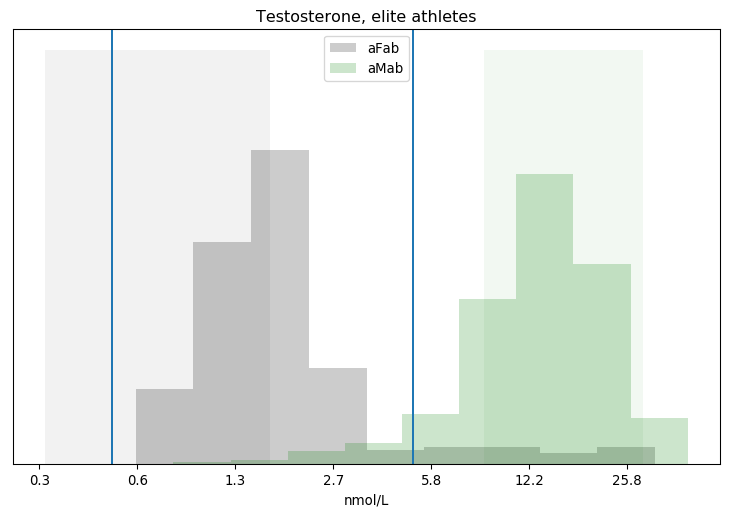
I've put vertical lines at both the 0.5 and 5 nmol/L cutoffs. There's a big difference between categories, but we can see clouds on the horizon: a substantial number of assigned-female athletes have greater than 5 nmol/L of testosterone in their bloodstream, while a decent number of assigned-male athletes have less. How many?
Segregating Athletes by Testosterone
Concentration  aFab  aMab
   > 5nmol/L    19   417
   < 5nmol/L   210    26
   = 5nmol/L     0     3

8.3% of assigned-female athletes have > 5nmol/L
5.8% of assigned-male athletes have < 5nmol/L
4.4% of athletes with > 5nmol/L are assigned-female
11.0% of athletes with < 5nmol/L are assigned-male
Looks like anywhere from 6-8% of athletes have testosterone levels that cross Rationality Rules' line. For comparison, maybe 1-2% of the general public has some level of gender dysphoria, though estimating exact figures is hard in the face of widespread discrimination and poor sex-ed in schools. Even that number is misleading, as the number of transgender athletes is substantially lower than 1-2% of the athletic population. The share of transgender athletes is irrelevant to this dataset anyway, as it was collected between 1996 and 1999, when no sporting agency had policies that allowed transgender athletes to openly compete.
That 6-8%, in other words, is entirely cisgender. This echoes one of Essence Of Thought's arguments: RR's 5nmol/L policy has far more impact on cis athletes than trans athletes, which could have catastrophic side-effects. Could is the operative word, though, because as of now we don't know anything about these athletes. Do >5nmol/L assigned-female athletes have bodies more like >5nmol/L assigned-male athletes than <5nmol/L assigned-female athletes? If so, then there's no problem. Equivalent body types are competing against each other, and outcomes are as fair as could be reasonably expected.
What, then, counts as an "equivalent" body type when it comes to sport?
One reasonable measure of equivalence is height. It's one of the stronger sex differences, and height is also correlated with longer limbs and greater leverage. Whether that's relevant to sports is debatable, but height and correlated attributes dominate Rationality Rules' list.
[19:07] In some events - such as long-distance running, in which hemoglobin and slow-twitch muscle fibers are vital - I think there's a strong argument to say no, [transgender women who transitioned after puberty] don't have an unfair advantage, as the primary attributes are sufficiently mitigated. But in most events, and especially those in which height, width, hip size, limb length, muscle mass, and muscle fiber type are the primary attributes - such as weightlifting, sprinting, hammer throw, javelin, netball, boxing, karate, basketball, rugby, judo, rowing, hockey, and many more - my answer is yes, most do have an unfair advantage.
Fortunately for both of us, most athletes in the dataset have a "valid" height, which I define as being at least 30cm tall.
Out of 693 athletes, 678 have valid height data.
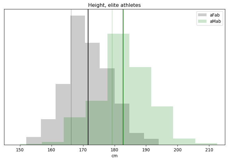
The faint vertical lines are for the mean adult height of Germans born in 1976, which should be a reasonable cohort to European athletes that were active between 1996 and 1999, while the darker lines are each category's mean. Athletes seem slightly taller than the reference average, but only by 2-5cm. The amount of overlap is also surprising, given that height is supposed to be a major sex difference. We actually saw less overlap with testosterone! Finally, the height distribution isn't quite Gaussian, there's a subtle bias towards the taller end of the spectrum.
Height is a pretty crude metric, though. You could pair any athlete with a non-athlete of the same height, and there's no way the latter would perform as well as the former. A better measure of sporting ability would be muscle mass. We shouldn't use the absolute mass, though: bigger bodies have more mass and need more force to accelerate as smaller bodies do, so height and muscle mass are correlated. We need some sort of dimensionless scaling factor which compensates.
And we have one! It's called the Body Mass Index, or BMI.
$$ BMI = \frac w {h^2}, $$
where \(w\) is a person's mass in kilograms, and \(h\) is a person's height in metres. Unfortunately, BMI is quite problematic. Partly that's because it is a crude measure of obesity. But part of that is because there are two types of tissue which can greatly vary, body fat and muscle, yet both contribute equally towards BMI.
That's all fixable. For one, some of the athletes in this dataset had their body fat measured. We can subtract that mass off, so their weight consists of tissues that are strongly correlated with height plus one that is fudgable: muscle mass. For two, we're not assessing these individual's health, we only want a dimensionless measure of muscle mass relative to height. For three, we're not comparing these individuals to the general public, so we're not restricted to using the general BMI formula. We can use something more accurate.
The oddity is the appearance of that exponent 2, though our world is three-dimensional. You might think that the exponent should simply be 3, but that doesn't match the data at all. It has been known for a long time that people don't scale in a perfectly linear fashion as they grow. I propose that a better approximation to the actual sizes and shapes of healthy bodies might be given by an exponent of 2.5. So here is the formula I think is worth considering as an alternative to the standard BMI:
$$ BMI' = 1.3 \frac w {h^{2.5}} $$
I can easily pop body fat into Nick Trefethen's formula, and get a better measure of relative muscle mass,
$$ \overline{BMI} = 1.3 \frac{ w - bf }{h^{2.5}}, $$
where \(bf\) is total body fat in kilograms. Individuals with excess muscle mass, relative to what we expect for their height, will have a high \(\overline{BMI}\), and vice-versa. And as we saw earlier, muscle mass is another of Rationality Rules' determinants of sporting performance.
Time for more number crunching.
Out of 693 athletes, 227 have valid adjusted BMIs.
                     663 have valid weights.
                     241 have valid body fat percentages.

Total Assigned-female Athletes = 239
 total with valid adjusted BMI = 86
  adjusted BMI, Mean     = 16.98
  adjusted BMI, Std.Dev  = 1.21
  adjusted BMI, Median   = 16.96

Total Assigned-male Athletes = 454
 total with valid adjusted BMI = 141
  adjusted BMI, Mean     = 20.56
  adjusted BMI, Std.Dev  = 1.88
  adjusted BMI, Median   = 20.28
The bad news is that most of this dataset lacks any information on body fat, which really cuts into our sample size. The good news is that we've still got enough to carry on. It also looks like there's a strong sex difference, and the distribution is pretty clustered. Still, a chart would help clarify the latter point.
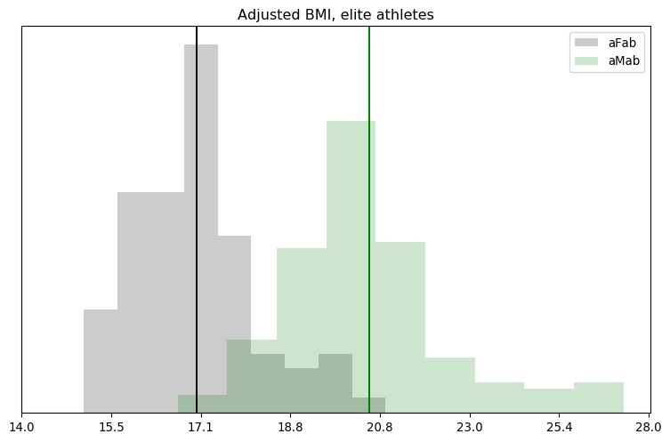
Whoops! There's more overlap and skew than I thought. Even in logspace, the results don't look Gaussian. We'll have to remember that for the next step.
Just looking at charts isn't going to solve this question, we need to do some sort of hypothesis testing. Fortunately, all the pieces I need are here. We've got our hypothesis, for instance:
Athletes with exceptional testosterone levels are more like athletes of the same sex but with typical testosterone levels, than they are of other athletes with a different sex but similar testosterone levels.
If you know me, you know that I'm all about the Bayes, and that gives us our methodology.
"Metric" is one of height or \(\overline{BMI}\), while "test group" is one of assigned-female athletes with >5nmol/L of serum testosterone or assigned-male athletes with <5nmol/L of serum testosterone. The Bayes Factor is simply
$$ \text{Bayes Factor} = \frac{ p(E \mid H_1) \cdot p(H_1) }{ p(E \mid H_2) \cdot p(H_2) } = \frac{ p(H_1 \mid E) }{ p(H_2 \mid E) }, $$
which means we need two hypotheses, not one. Fortunately, I've phrased the hypothesis to make it easy to negate: athletes with exceptional testosterone levels are less like athletes of the same sex but with typical testosterone levels, than they are of other athletes with a different sex but similar testosterone levels. We'll call this new hypothesis \(H_2\), and the original \(H_1\). Bayes factors greater than 1 mean \(H_1\) is more likely than \(H_2\), and vice-versa.
Calculating all that would be easy if I was using Stan or PyMC3, but I ran into problems translating the former's probability distributions into charts, and I don't have any experience with the latter. My next choice, emcee, forces me to manually convolve two posterior distributions. Annoying, but not difficult.
That just leaves one thing left: what models are we going to use? The obvious choice for height is the Gaussian distribution, as from previous research we know it's a great model.
Fitting the height of lT aFab athletes to a Gaussian distribution ...
     0: (-980.322471) mu=150.000819, sigma=15.000177
    64: (-710.417497) mu=169.639051, sigma=8.579088
   128: (-700.539260) mu=171.107358, sigma=7.138832
   192: (-700.535241) mu=171.154151, sigma=7.133279
   256: (-700.540692) mu=171.152701, sigma=7.145515
   320: (-700.552831) mu=171.139668, sigma=7.166857
   384: (-700.530969) mu=171.086422, sigma=7.094077
    ML: (-700.525284) mu=171.155240, sigma=7.085777
median: (-700.525487) mu=171.134614, sigma=7.070993
Alas, emcee also lacks a good way to assess model fitness. One crude metric is look at the progression of the mean fitness; if it grows and then stabilizes around a specific value, as it does here, we've converged on something. Another is to compare the mean, median, and maximal likelihood of the posterior; if they're about equally likely, we've got a fuzzy caterpillar. Again, that's also true here.
As we just saw, though, charts are a better judge of fitness than a handful of numbers.

If you were wondering why I didn't make much of a fuss out of the asymmetry in the height distribution, it's because I've already seen this graph. A good fit isn't necessarily the best though, and I might be able to get a closer match by incorporating the sport each athlete played.
            Assigned-female Athletes
         sport              below/above 171cm
           Power lifting:  1 / 0
              Basketball:  2 /12
                Football:  0 / 0
                Swimming: 41 /49
                Marathon:  0 / 1
                Canoeing:  1 / 0
                  Rowing:  9 /13
    Cross-country skiing:  8 / 1
           Alpine skiing: 11 / 1
          Weight lifting:  7 / 0
                    Judo:  0 / 0
                   Bandy:  0 / 0
              Ice Hockey:  0 / 0
                Handball: 12 /17
         Track and field: 22 /27
Basketball attracts tall people, unsurprisingly, while skiing seems to attract shorter people. This could be the cause of that asymmetry. It's no guarantee that I'll actually get a better fit, though, as I'm also dramatically cutting the number of datapoints to fit to. The model's uncertainty must increase as a result, and that may be enough to dilute out any increase in fitness. I'll run those numbers for the paper, but for now the Gaussian model I have is plenty good.
Fitting the height of hT aMab athletes to a Gaussian distribution ...
     0: (-2503.079578) mu=150.000061, sigma=15.001179
    64: (-1482.315571) mu=179.740851, sigma=10.506003
   128: (-1451.789027) mu=182.615810, sigma=8.620333
   192: (-1451.748336) mu=182.587979, sigma=8.550535
   256: (-1451.759883) mu=182.676004, sigma=8.546410
   320: (-1451.746697) mu=182.626918, sigma=8.538055
   384: (-1451.747266) mu=182.580692, sigma=8.534070
    ML: (-1451.746074) mu=182.591047, sigma=8.534584
median: (-1451.759295) mu=182.603231, sigma=8.481894
We get the same results when fitting the model to >5 nmol/L assigned-male athletes. The log likelihood, that number in brackets, is a lot lower for these athletes, but that number is roughly proportional to the number of samples. If we had the same degree of model fitness but doubled the number of samples, we'd expect the log likelihood to double. And, sure enough, this dataset has roughly twice as many assigned-male athletes as it does assigned-female athletes.
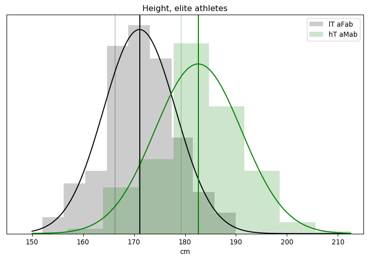
The updated charts are more of the same.
Unfortunately, adjusted BMI isn't nearly as tidy. I don't have any prior knowledge that would favour a particular model, so I wound up testing five candidates: the Gaussian, Log-Gaussian, Gamma, Weibull, and Rayleigh distributions. All but the first needed an offset parameter to get the best results, which has the same interpretation as last time.
Fitting the adjusted BMI of hT aMab athletes to a Gaussian distribution ...
     0: (-410.901047) mu=14.999563, sigma=5.000388
   384: (-256.474147) mu=20.443497, sigma=1.783979
    ML: (-256.461460) mu=20.452817, sigma=1.771653
median: (-256.477475) mu=20.427138, sigma=1.781139
Fitting the adjusted BMI of hT aMab athletes to a Log-Gaussian distribution ...
     0: (-629.141577) mu=6.999492, sigma=2.001107, off=10.000768
   384: (-290.910651) mu=3.812746, sigma=1.789607, off=16.633741
   ML: (-277.119315) mu=3.848383, sigma=1.818429, off=16.637382
median: (-288.278918) mu=3.795675, sigma=1.778238, off=16.637076
Fitting the adjusted BMI of hT aMab athletes to a Gamma distribution ...
    0: (-564.227696) alpha=19.998389, beta=3.001330, off=9.999839
   384: (-256.999252) alpha=15.951361, beta=2.194827, off=13.795466
ML    : (-248.056301) alpha=8.610936, beta=1.673886, off=15.343436
median: (-249.115483) alpha=12.411010, beta=2.005287, off=14.410945
Fitting the adjusted BMI of hT aMab athletes to a Weibull distribution ...
    0: (-48865.772268) k=7.999859, beta=0.099877, off=0.999138
  384: (-271.350390) k=9.937527, beta=0.046958, off=0.019000
   ML: (-270.340284) k=9.914647, beta=0.046903, off=0.000871
median: (-270.974131) k=9.833793, beta=0.046947, off=0.011727
Fitting the adjusted BMI of hT aMab athletes to a Rayleigh distribution ...
    0: (-3378.099000) tau=0.499136, off=9.999193
  384: (-254.717778) tau=0.107962, off=16.378780
   ML: (-253.012418) tau=0.110751, off=16.574934
median: (-253.092584) tau=0.108740, off=16.532576

Looks like the Gamma distribution is the best of the bunch, though only if you use the median or maximal likelihood of the posterior. There must be some outliers in there that are tugging the mean around. Visually, there isn't too much difference between the Gaussian and Gamma fits, but the Rayleigh seems artificially sharp on the low end. It's a bit of a shame, the Gamma distribution is usually related to rates and variance so we don't have a good reason for applying it here, other than "it fits the best." We might be able to do better with a per-sport Gaussian distribution fit, but for now I'm happy with the Gamma.
Time to fit the other pool of athletes, and chart it all.
Fitting the adjusted BMI of lT aFab athletes to a Gamma distribution ...
    0: (-127.467934) alpha=20.000007, beta=3.000116, off=9.999921
   384: (-128.564564) alpha=15.481265, beta=3.161022, off=12.654149
ML    : (-117.582454) alpha=2.927721, beta=1.294851, off=14.713479
median: (-120.689425) alpha=11.961847, beta=2.836153, off=13.008723
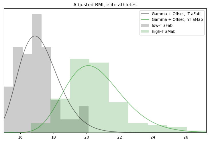
Those models look pretty reasonable, though the upper end of the assigned-female distribution could be improved on. It's a good enough fit to get some answers, at least.
It's easier to combine step 3, applying the model, with step 5, calculating the Bayes Factor, when writing the code. The resulting Bayes Factor has a probability distribution, as the uncertainty contained in the posterior contaminates it.
Summary of the BF distribution, for the height of >5nmol/L aFab athletes
         n       mean   geo.mean         5%        16%        50%        84%        95%
        19      10.64       5.44       0.75       1.76       5.66      17.33      35.42

Percentage of BF's that favoured the primary hypothesis: 92.42%
Percentage of BF's that were 'decisive': 14.17%
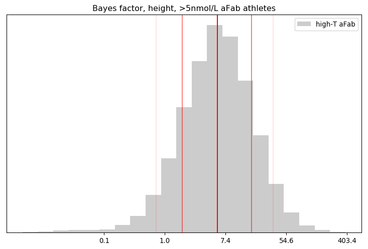
That looks a lot like a log-Gaussian distribution. The arthithmetic mean fails us here, thanks to the huge range of values, so the geometric mean and median are better measures of central tendency.
The best way I can interpret this result is via an eight-sided die: our credence in the hypothesis that >5nmol/L aFab athletes are more like their >5nmol/L aMab peers than their <5nmol/L aFab ones is similar to the credence we'd place on rolling a one via that die, while our credence on the primary hypothesis is similar to rolling any other number except one. About 92% of the calculated Bayes Factors were favourable to the primary hypothesis, and about 16% of them crossed the 19:1 threshold, a close match for the asserted evidential bar in science.
That's strong evidence for a mere 19 athletes, though not quite conclusive. How about the Bayes Factor for the height of <5nmol/L aMab athletes?
Summary of the BF distribution, for the height of <5nmol/L aMab athletes
         n       mean   geo.mean         5%        16%        50%        84%        95%
        26   4.67e+21   3.49e+18   5.67e+14   2.41e+16   5.35e+18   4.16e+20   4.61e+21

Percentage of BF's that favoured the primary hypothesis: 100.00%
Percentage of BF's that were 'decisive': 100.00%
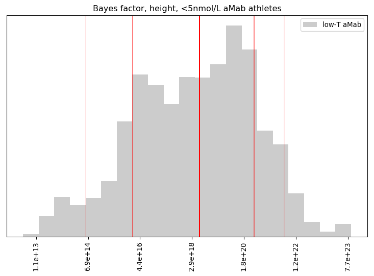
Wow! Even with 26 data points, our primary hypothesis was extremely well supported. Betting against that hypothesis is like betting a particular person in the US will be hit by lightning three times in a single year!
That seems a little too favourable to my view, though. Did something go wrong with the mathematics? The simplest check is to graph the models against the data they're evaluating.
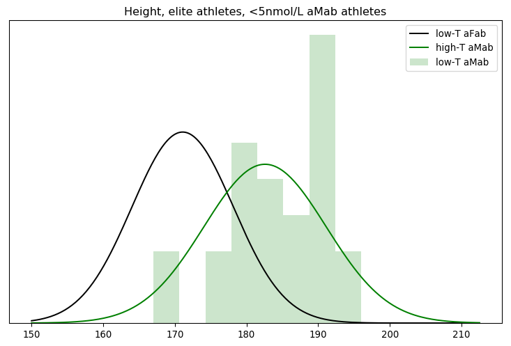
Nope, the underlying data genuinely is a better fit for the high-testosterone aMab model. But that good of a fit? In linear space, we multiply each of the individual probabilities to arrive at the Bayes factor. That's equivalent to raising the geometric mean to the nth power, where n is the number of athletes. Since n = 26 here, even a geometric mean barely above one can generate a big Bayes factor.
26th root of the median Bayes factor of the high-T aMab model applied to low-T aMab athletes: 5.2519
26th root of the Bayes factor for the median marginal: 3.6010
Note that the Bayes factor we generate by using the median of the marginal for each parameter isn't as strong as the median Bayes factor in the above convolution. That's simply because I'm using a small sample from the posterior distribution. Keeping more samples would have brought those two values closer together, but also greatly increased the amount of computation I needed to do to generate all those Bayes factors.
With that check out of the way, we can move on to \(\overline{BMI}\).
Summary of the BF distribution, for the adjusted BMI of >5nmol/L aFab athletes
         n       mean   geo.mean         5%        16%        50%        84%        95%
         4   1.70e+12   1.06e+05   2.31e+02   1.60e+03   4.40e+04   3.66e+06   3.99e+09

Percentage of BF's that favoured the primary hypothesis: 100.00%
Percentage of BF's that were 'decisive': 99.53%
Percentage of non-finite probabilities, when applying the low-T aFab model to high-T aFab athletes: 0.00%
Percentage of non-finite probabilities, when applying the high-T aMab model to high-T aFab athletes: 10.94%
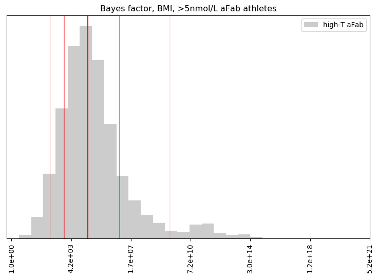
This distribution is much stranger, with a number of extremely high BF's that badly skew the mean. The offset contributes to this, with 7-12% of the model posteriors for high-T aMab athletes assigning a zero percent likelihood to an adjusted BMI. Those are excluded from the analysis, but they suggest the high-T aMab model poorly describes high-T aFab athletes.
Our credence in the primary hypothesis here is similar to our credence that an elite golfer will not land a hole-in-one on their next shot. That's surprisingly strong, given we're only dealing with four datapoints. More data may water that down, but it's unlikely to overcome that extreme level of credence.
Summary of the BF distribution, for the adjusted BMI of <5nmol/L aMab athletes
         n       mean   geo.mean         5%        16%        50%        84%        95%
         9   6.64e+35   2.07e+22   4.05e+12   4.55e+16   6.31e+21   7.72e+27   9.81e+32

Percentage of BF's that favoured the primary hypothesis: 100.00%
Percentage of BF's that were 'decisive': 100.00%
Percentage of non-finite probabilities, when applying the high-T aMab model to low-T aMab athletes: 0.00%
Percentage of non-finite probabilities, when applying the low-T aFab model to low-T aMab athletes: 0.00%

The hypotheses' Bayes factor for the adjusted BMI of low-testosterone aMab athletes is much better behaved. Even here, the credence is above three-lightning-strikes territory, pretty decisively favouring the hypothesis.
Our final step would normally be to combine all these individual Bayes factors into a single one. That involves multiplying them all together, however, and a small number multiplied by a very large one is an even larger one. It isn't worth the effort, the conclusion is pretty obvious.
Our primary hypothesis is on quite solid ground: Athletes with exceptional testosterone levels are more like athletes of the same sex but with typical testosterone levels, than they are of other athletes with a different sex but similar testosterone levels. If we divide up sports by testosterone level, then, roughly 6-8% of assigned-male athletes will wind up in the <5 nmol/L group, and about the same share of assigned-female athletes will be in the >5 nmol/L group. Note, however, that it doesn't follow that 6-8% of those in the <5 nmol/L group will be assigned-male. About 41% of the athletes at the 2018 Olymics were assigned-female, for instance. If we fix the rate of exceptional testosterone levels at 7%, and assume PyeongChang's rate is typical, a quick application of Bayes' theorem reveals
$$ \begin{align} p( \text{aMab} \mid \text{<5nmol/L} ) &= \frac{ p( \text{<5nmol/L} \mid \text{aMab} ) p( \text{aMab} ) }{ p( \text{<5nmol/L} \mid \text{aMab} ) p( \text{aMab} ) + p( \text{<5nmol/L} \mid \text{aFab} ) p( \text{aFab} ) } \\ {} &= \frac{ 0.07 \cdot 0.59 }{ 0.07 \cdot 0.59 + 0.93 \cdot 0.41 } \\ {} &\approx 9.8\% \end{align} $$
If all those assumptions are accurate, about 10% of <5 nmol/L athletes will be assigned-male, more-or-less matching the number I calculated way back at the start. In sports where performance is heavily correlated with height or \(\overline{BMI}\), then, the 10% of assigned-male athletes in the <5 nmol group will heavily dominate the rankings. The odds of a woman earning recognition in this sport are negligible, leading many of them to drop out. This increases the proportion of men in that sport, leading to more domination of the rankings, more women dropping out, and a nasty feedback loop.
Conversely, about 5% of >5nmol/L athletes will be assigned-female. In a heavily-correlated sport, those women will be outclassed by the men and have little chance of earning recognition for their achievements. They have no incentive to compete, so they'll likely drop out or avoid these sports as well.
In events where physicality has less or no correlation with sporting performance, these effects will be less pronounced or non-existent, of course. But this still translates into fewer assigned-female athletes competing than in the current system.
But it gets worse! We'd also expect an uptick in the number of assigned-female athletes doping, primarily with testosterone inhibitors to bring themselves just below the 5nmol/L line. Alternatively, high-testosterone aFab athletes may inject large doses of testosterone to bulk up and remain competitive with their assigned-male competitors.
By dividing up testosterone levels into only two categories, sporting authorities are implicitly stating that everyone within those categories is identical. A number of athletes would likely go to court to argue that boosting or inhibiting testosterone should be legal, provided they do not cross the 5nmol/L line. If they're successful, then either the rules around testosterone usage would be relaxed, or sporting authorities would be forced to subdivide these groups further. This would lead to an uptick in testosterone doping among all athletes, not just those assigned female.
Notice that assigned-male athletes don't have the same incentives to drop out, and in fact the low-testosterone subgroup may even be encouraged to compete as they have an easier path to sporting fame and glory. Sports where performance is heavily correlated with height or \(\overline{BMI}\) will come to be dominated by men.
[1:15] In a nutshell, I find the arguments and logic that currently permit transgender women to compete against biological women to be remarkably flawed, and I’m convinced that unless quickly rectified, this will KILL women’s sports.
[14:00] I don’t want to see the day when women’s athletics is dominated by Y chromosomes, but without a change in policy, that is precisely what’s going to happen.
It's rather astounding. Transgender athletes are a not a problem, on several levels; as I've pointed out before, they've been allowed to compete in the category they identify for over a decade in some places, and yet no transgender athlete has come to dominate any sport. The Olympics has held the door open since 2004, and not a single transgender athlete has ever openly competed as a transgender athlete. Rationality Rules, like other transphobes, is forced to cherry-pick and commit lies of omission among a handful of examples, inflating them to seem more significant than they actually are.
In response to this non-existent problem, Rationality Rules' proposed solution would accomplish the very thing he wants to avoid! You don't get that turned around if you're a rational person with a firm grasp on the science.
No, this level of self-sabotage is only possible if you're a clueless bigot who's ignorant of the relevant science, and so frightened of transgender people that your critical thinking skills abandon you. The vast difference between what Rationality Rules claims the science says, and what his own citations say, must be because he knows that if he puts on a good enough act nobody will check his work. Everyone will walk away assuming he's rational, rather than a scared, dishonest loon.
It's hard to fit any other conclusion to the data.